Numerical Optimization VI: Optimization and linear algebra

Today

Linear algebra formulation

solving system of equation

Bringing back optimization

solving over constrained system of equation

Mobile problem

Someone provided us with 6 weights and 3 rods. We need to calculate the positions of suspension points to have a balanced system.

If the system is in equilibrium, torque must be zero at every pivot point $\begin{aligned} w_1 x_1 - (w_2 + w_3 + w_4 + w_5 + w_6) x_2 &=& 0 \\ w_3 x_3 - (w_4 + w_5 + w_6) x_4 &=& 0 \\ w_5 x_5 - w_6 x_6 &=& 0 \end{aligned}$

Let’s define $w_{26}=w_2 + w_3 + w_4 + w_5+w_6$ and $w_{46}=w_4+w_5+w_6$

$\begin{aligned} w_1 x_1 - w_{26} x_2 &=& 0 \\ w_3 x_3 - w_{46} x_4 &=& 0 \\ w_5 x_5 - w_6 x_6 &=& 0 \\ \end{aligned}$

We need 3 more equations. Let’s constrain the length of every rod $\begin{aligned} x_1 + x_2 &=& L_{12} \\ x_3 + x_4 &=& L_{34} \\ x_5 + x_6 &=& L_{56} \end{aligned}$

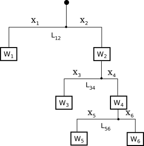
Mobile scketch

Mobile problem continued

Mobile scketch

$\begin{aligned} w_1 x_1 - w_{26} x_2 &=& 0 \\ w_3 x_3 - w_{46} x_4 &=& 0 \\ w_5 x_5 - w_6 x_6 &=& 0 \\ x_1 + x_2 &=& L_{12} \\ x_3 + x_4 &=& L_{34} \\ x_5 + x_6 &=& L_{56} \end{aligned}$

$\begin{aligned} \begin{pmatrix} w_1 & -w_{26} & 0 & 0 & 0 & 0 \\ 0 & 0 & w_3 & -w_{46} & 0 & 0 \\ 0 & 0 & 0 & 0 & w_5 & -w_6 \\ 1 & 1 & 0 & 0 & 0 & 0 \\ 0 & 0 & 1 & 1 & 0 & 0 \\ 0 & 0 & 0 & 0 & 1 & 1 \end{pmatrix} \begin{pmatrix} x_1 \\ x_2 \\ x_3 \\ x_4 \\ x_5 \\ x_6 \end{pmatrix} = \begin{pmatrix} 0 \\ 0 \\ 0 \\ L_{12} \\ L_{34} \\ L_{56} \end{pmatrix} \end{aligned}$

$\begin{aligned} \sum_j A_{ij} x_j = B_i \to {\mathbf A} {\mathbf x} = {\mathbf B} \end{aligned}$

Bold marks matrices. Vector such as ${\mathbf x}$ and ${\mathbf B}$ are matrices too (1D).

Python has a lot of built-in functions to solve problems in this form

Linear Algebra inverse matrix method

$\begin{aligned} {\mathbf A} {\mathbf x} &=& {\mathbf B} \\ {\mathbf A^{-1}} {\mathbf A} {\mathbf x} &=& {\mathbf A^{-1}}{\mathbf B} \\ {\mathbf x} &=& {\mathbf A^{-1}}{\mathbf B} \end{aligned}$

Analytical solution ${\mathbf x} = {\mathbf A^{-1}}{\mathbf B}$ exists only if $\text{determinant}({\mathbf A}) \ne 0$

Remember that ${\mathbf A^{-1}} {\mathbf A} = {\mathbf A} {\mathbf A^{-1}} = {\mathbf I}$ , where ${\mathbf I}$ is the unity matrix.

Python’s straight forward implementation (not the fastest)

import numpy as np

# define A and B marices

invA = np.linalg.inv(A)

# Pay attention @ is not the same as *

# @ also  is matrix multiplication by Linear Algebra rules

# *  is the element wise multiplication

x = invA @ B

Inverting matrix is computationally expensive!

Python’s faster way by using equation solver directly (recommended)

import numpy as np

# define A and B marices

invA = inv(A)
x = np.linalg.solve(A, B)

Examples

$\begin{aligned} 2 x_1 + 3 x_2 &= 8 \\ 5 x_1 + 1 x_2 &= 7 \end{aligned}$

${\mathbf A} {\mathbf x} = {\mathbf B}$

$\begin{aligned} \begin{pmatrix} 2 & 3\\ 5 & 1 \end{pmatrix} \cdot \begin{pmatrix} x_1 \\ x_2 \end{pmatrix} = \begin{pmatrix} 8 \\ 7 \end{pmatrix} \end{aligned}$

import numpy as np
A = np.array([[ 2, 3], [5, 1]])
B = np.array([[8], [7]])
invA = np.linalg.inv(A)
x = invA @ B

In [9]: invA
Out[9]:
array([[-0.07692308,  0.23076923],
       [ 0.38461538, -0.15384615]])

In [10]: x
Out[10]:
array([[1.],
       [2.]])

import numpy as np
A = np.array([[ 2, 3], [5, 1]])
B = np.array([[8], [7]])
x = np.linalg.solve(A, B)

In [12]: x
Out[12]:
array([[1.],
       [2.]])

# check

In [15]: A @ x
Out[15]:
array([[8.],
       [7.]])

Recall the mobile problem

If $w_1=20$ , $w_2=5$ , $w_3=3$ , $w_4=7$ , $w_5=2$ , $w_6=3$ , $L_{12}=2$ , $L_{34}=1$ , and $L_{56}=3$ , then $w_{26}=20$ and $w_{46}=12$ .

$\begin{aligned} \begin{pmatrix} 20 & -20 & 0 & 0 & 0 & 0 \\ 0 & 0 & 3 & -12 & 0 & 0 \\ 0 & 0 & 0 & 0 & 2 & -3 \\ 1 & 1 & 0 & 0 & 0 & 0 \\ 0 & 0 & 1 & 1 & 0 & 0 \\ 0 & 0 & 0 & 0 & 1 & 1 \end{pmatrix} \begin{pmatrix} x_1 \\ x_2 \\ x_3 \\ x_4 \\ x_5 \\ x_6 \end{pmatrix} = \begin{pmatrix} 0 \\ 0 \\ 0 \\ 2 \\ 1 \\ 3 \end{pmatrix} \end{aligned}$

import numpy as np

A=np.array([
[20, -20, 0, 0, 0, 0],
[0, 0, 3, -12, 0, 0],
[0, 0, 0, 0, 2, -3],
[1, 1, 0, 0, 0, 0],
[0, 0, 1, 1, 0, 0],
[0, 0, 0, 0, 1, 1],
])
B= np.array([[0], [0], [0], [2], [1], [3] ])

x=np.linalg.inv(A) @ B

In [33]: x
Out[33]:
array([[1. ],
       [1. ],
       [0.8],
       [0.2],
       [1.8],
       [1.2]])

Check

In [32]: A @ x - B
Out[32]:
array([[0.0000000e+00],
       [0.0000000e+00],
       [0.0000000e+00],
       [0.0000000e+00],
       [0.0000000e+00],
       [4.4408921e-16]])

To do or not to do the inverse matrix calculation

Solutions based on the inverse matrix calculation involve extra steps (unnecessary for solution) and, thus, are slower

However, it is handy to calculate the inverse matrix in advance if you solve ${\mathbf A} {\mathbf x} = {\mathbf B}$ for different ${\mathbf B}$ with the same ${\mathbf A}$ .

Reformulating via optimization problem

We can say that

${\mathbf A} {\mathbf x} = {\mathbf B}$

is equivalent to

find ${\mathbf x}$ which minimizes $|{\mathbf A} {\mathbf x} - {\mathbf B}|$

In python it can be done via

import numpy as np
A = np.array([[ 2, 3], [5, 1]])
B = np.array([[8], [7]])

sol = np.linalg.lstsq(A, B)
x = sol[0]
 
In [40]: x
Out[40]:
array([[1.],
       [2.]])

Optimization solver benefits

Sounds useless but it allows to solve over constrained problems like

$\begin{aligned} 4x = 3 \\ 5x = 2 \end{aligned}$

Very common in physics. Mentally replace $x \to R$

$\begin{aligned} I_1 R = V_1 \\ I_2 R = V_2 \\ \cdots \\ I_n R = V_n \\ \end{aligned}$

import numpy as np
A=np.array([ [4], [5] ])

B=np.array([ [3], [2] ])

sol = np.linalg.lstsq(A, B)
x = sol[0]

In [44]: x
Out[44]: array([[0.53658537]])