Today

Combinatorial optimization in multiple dimensions

• Revisiting Back pack problem
  • global optimum with brute force
  • optimum search with annealing
• Traveling salesman problem

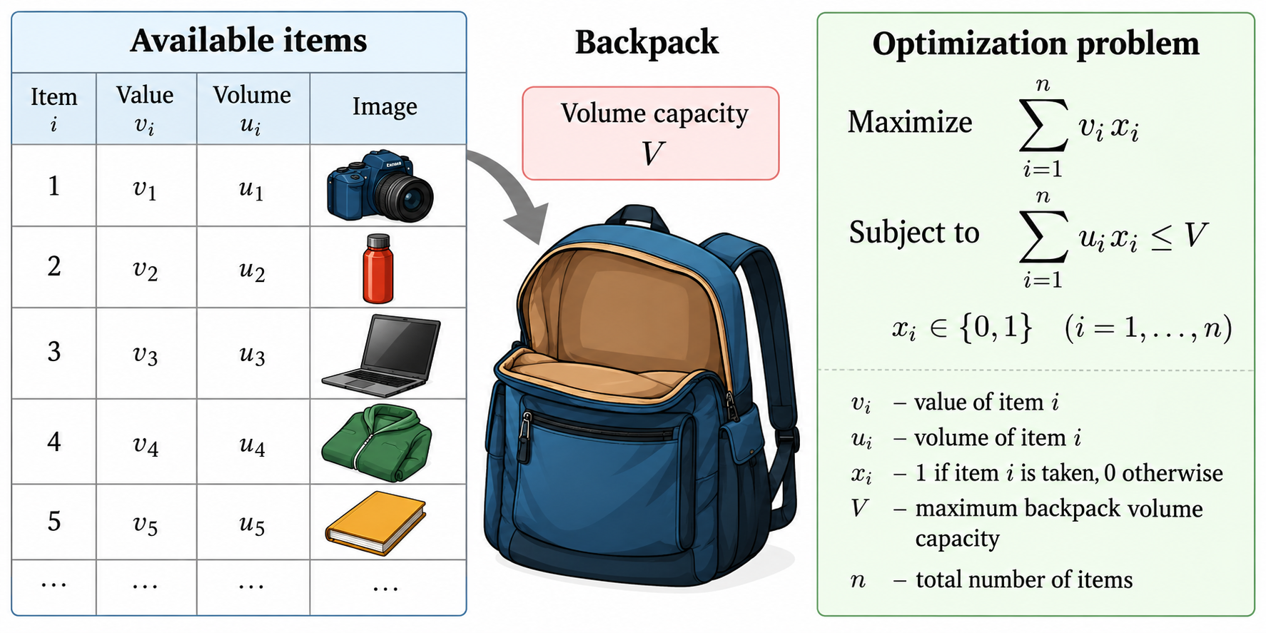
Revisiting Backpack problem

For simplicity, we will assume that every item occurs only once.

Our job is to maximize $$\begin{aligned} E(\vec{x}) = \sum \text{value}_i x_i = \overrightarrow{\text{values}} \cdot \vec{x} \end{aligned}$$ Subject to the following constraints $$\begin{aligned} \sum \text{volume}_i x_i = \overrightarrow{\text{volumes}} \cdot \vec{x} \le \text{BackpackSize} \end{aligned}$$

$\vec{x}$ is a combination of zeros and ones $\vec{x}=[0,1,0,1,\cdots,1,1,0,1,1]$.

Backpack illustration (generated by ChatGPT)

Backpack optimization with binary encoding: test run

• My office computer sorts through 20 items in 4.4 seconds, but 30 items would take 1000 times longer, i.e. about 75 minutes to solve. And my home computer is factor of 5 slower.

#!/usr/bin/env python3
import numpy as np

def backpack_binary(max_capacity, values, volumes):
    """ Solve backpack problem using binary coding approach."""
    n = len(values)
    max_value = 0
    best_combination = np.zeros(n, dtype=int)

# Try all possible combinations using binary representation

# From 0 to 2^n - 1 (all possible binary numbers with n bits)

for i in range(2**n):
        selected_items = np.zeros(n, dtype=int)
        
        code = bin(i)[2:].zfill(n) # string representing bits
        for i,s in enumerate(code):
            selected_items[i] = 1 if s=="1" else 0
        total_volume = np.sum(volumes * selected_items)
        total_value = np.sum(values * selected_items)

        if total_volume <= max_capacity:
            if total_value > max_value:
                max_value = total_value
                best_combination = selected_items.copy()
    return max_value, best_combination


def print_solution(values, volumes, max_capacity, max_value, selected_items):
    print(f"Backpack Capacity: {max_capacity}")
    print(f"Maximum Value: {max_value}")
    print(f"Selected Items: {selected_items}")
    print(f"{values=}")
    print(f"{volumes=}")
    print(f"Total number of objects: {len(values)}")


if __name__ == "__main__":
    print("====== Example 1 ===========")
    values1 = np.array([12, 10, 20, 15], dtype=int)
    volumes1 = np.array([2, 1, 3, 2], dtype=int)
    max_capacity1 = 5
    
    max_val1, selected1 = backpack_binary(max_capacity1, values1, volumes1)
    print_solution(values1, volumes1, max_capacity1, max_val1, selected1)
    
    print("====== Example 2 ===========")
    N=20
    values2 = (100*np.random.uniform(size=(N))).astype(int)
    volumes2 = (80*np.random.uniform(size=(N))).astype(int)
    max_capacity2 = 50
    
    import time
    t0 = time.time()
    max_val2, selected2 = backpack_binary(max_capacity2, values2, volumes2)
    print_solution(values2, volumes2, max_capacity2, max_val2, selected2)
    print(f"Execution time: {time.time() - t0}")

For realization of this algorithm, have a look at the backpack_binaray.py

Backpack optimization with simulated annealing

As with every optimization there are two challenges

Construction of the cost function

• note that we have a challenge of implementing backpack capacity

Penalty should have the following property

• grows with the over sizing demand
• ideally be smooth and monotonic
• should be zero if items fit

Update of the search point

We will toggle a random $x_i$, it is handy to select position with i=np.random.randint(0,high=N)

AI coded solution for backpack optimization with simulated annealing

We use prompt

Read 'backpack_binaray.py' and modify it to find the best combo with simulated annealing
algorithm. Use minimization paradigm, i.e. negate maximum value.
Use parameters Tstart, coolingRate, and Niterations.

If backpack items exceed max_capacity, add penalty to value proportional to oversize.

Save resulted script in 'backpack_annealing.py'

the outcome is in backpack_annealing.py

Brute force vs simulated annealing (AI generated comparison)

To compare two method, we use the follow up prompt (in the same context)

Write script which compares outcomes of binary and annealing versions,
encode threshold for not running binary search and put it to 15.
Also add relative value to the table.

the outcome script is compare_backpack_solutions.py

It produces the following table (after setting the threshold to 20)

Example: Traveling salesman problem

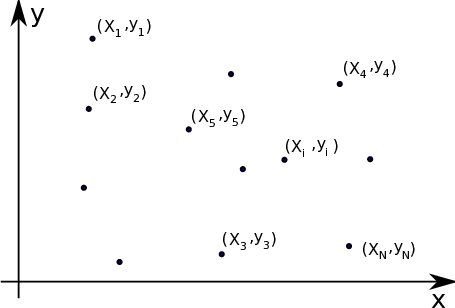
• Suppose that you have N cities (with given coordinates) to visit.
• A salesman starts in the city 1 and need to be in the $N_{th}$ city at the end of a route.
• The salesman must visit every city and do it only once.
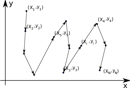
• Find the shortest route which satisfies the above conditions.

This problem has a lot of connections to the real world. Every time you ask your GPS to find a route, the GPS unit has to solve a similar problem. The traces placement on a printed circuit board is essentially the same problem, as well.

Possible brute force solution

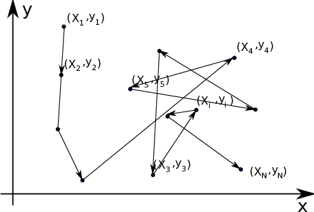
• Try every possible combination (permutation) of the cities ordering and choose the best one.
• Since the ends points are fixed, the combinatorial complexity of this problem $$\begin{aligned} (N-2)! \end{aligned}$$

This grows very fast with the $N$ increase.

• Will work for the modest cities number $N \le 10$ or may be slightly more.
• But even for a moderate $N=100$ it is hopeless. $100! \approx 10^158$ which is larger than number of atoms in the universe by a HUGE margin.

Permutation generating algorithm

See “The Art of Computer Programming, Volume 4 : Generating All Tuples and Permutations” by Donald Knuth for the discussion of the algorithm. The method below goes back to 14th century India.

1. Start with the set sorted in the ascending order, i.e. $p=[1,2,3,4, \cdots, N-2, N-1, N]$
2. Find the largest index $k$ such that $p(k) < p(k + 1)$.
   • If no such index exists, the permutation is the last permutation.
3. Find the largest index $l$ such that $p(k) < p(l)$.
   • There is at least one $l=k+1$
4. Swap $p(k)$ with $p(l)$.
5. Reverse the sequence from $p(k + 1)$ up to and including the final element $p(end)$.
6. We have a new permutation. If we need another, repeat from the step 2.

Luckily python already has it implemented

import itertools
items = [1, 2, 3]
perms = list(itertools.permutations(items))

In [59]: perms
Out[59]: [(1, 2, 3), (1, 3, 2), (2, 1, 3), (2, 3, 1), (3, 1, 2), (3, 2, 1)]

AI coded solution for traveling salesman brute force optimization

We use prompt

Write a traveling salesman path searching as `def traveling_salesman_permutations(coord)`,
for a person who always start in 1st city
and end in the last city. Cities coordinate will be encoded in Nx2 array where 1st column is
x and 2nd is y. Solution should return array which lists cities in order of visits.
Implement it via permutation using `intertools.permutations`. When ever possible use numpy
array operations.

Measure and output the path searching time.

Add visualization of the best path mark with different color the 1st and the last city.
And prepare example with 10 cities.

Save outcome to file 'salesman.py'

the outcome is in salesman.py

10 cities path optimization takes about 1.2 seconds on my old home computer.

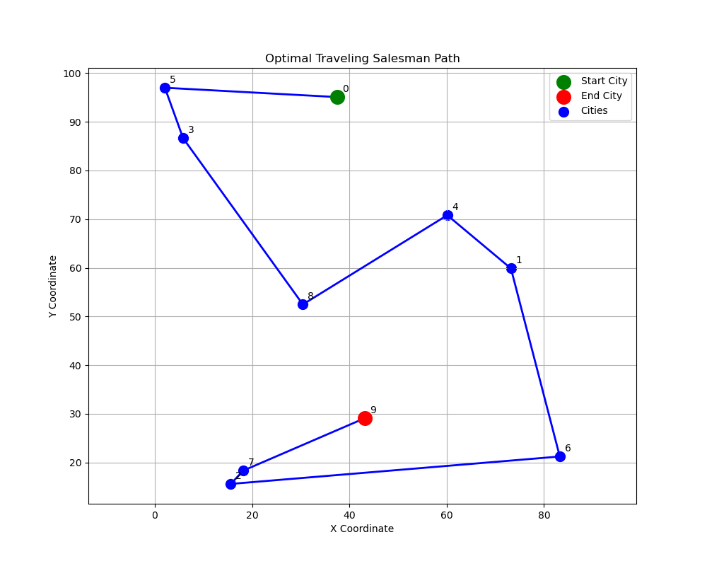
10 cities optimal path

AI coded solution for traveling salesman with simulated annealing

Prompting

use 'salesman.py' as a base and implement the path search with simulated annealing algorithm.
Save resulting script to 'salesman_annealing.py'

the outcome script is salesman_annealing.py

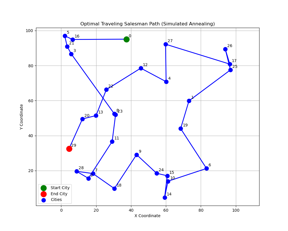
30 cities path generated with $10^5$ iterations and slow cooling rate