Numerical Optimization III: Gradient Descent
Eugeniy E. Mikhailov and Greg Bentsen
Logistics and Agenda
Homework 5 due Monday Oct 26 at 11:59pm
Midterm 2
- Take-home posted Monday Oct 26
- In-class exam Monday Nov 2
Agenda
- This week: Optimization in multiple dimensions
- Next week: Advanced optimization, combinatoric optimization,
machine learning
Today
Optimization in multiple dimensions
- Gradient descent optimization
- Multi-start optimization + AI demo
- Advanced techniques
- Nelder-Mead (derivative-free)
- Simulated annealing
Goal: Efficiently navigate the global energy
landscape.
Hunt for global minimum (but often get stuck in local minima
instead).
Where we left off
Given adjustable parameters
,
minimize the objective function
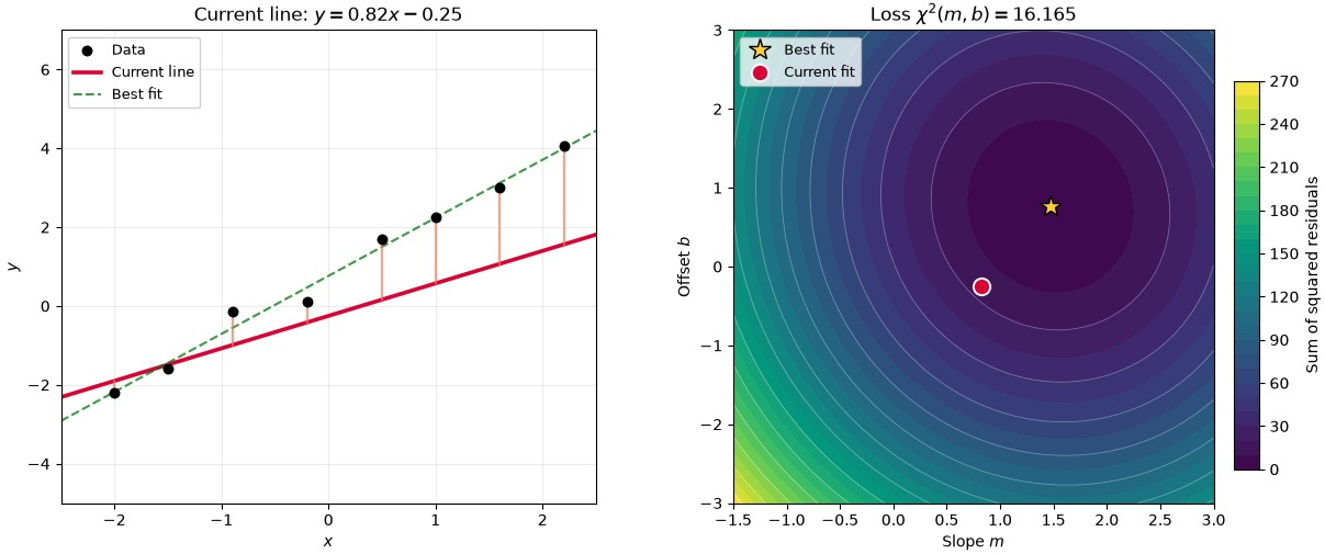
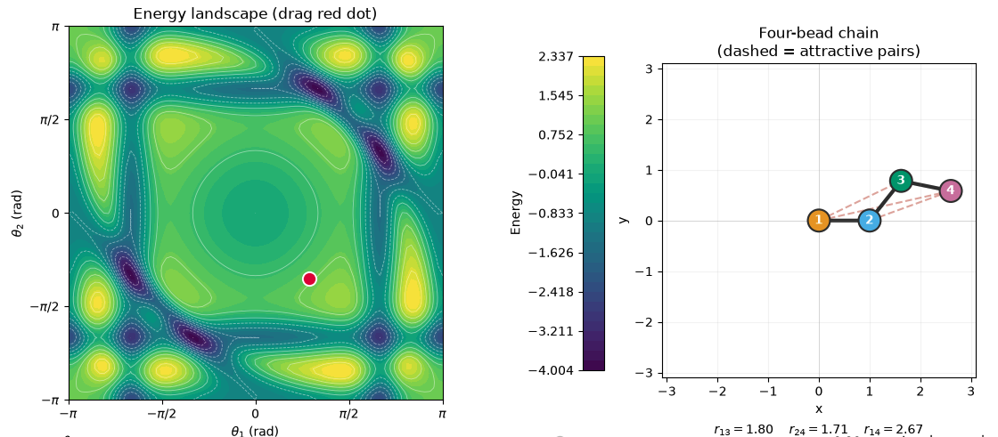
Two examples from last time:
- Linear regression:
- parameters
- objective
- Four-bead protein:
- parameters
- objective
Question: How do we find the bottom of a landscape
without scanning every point?
Gradient-Based Optimization
The gradient: which way is uphill?
For
,
define the gradient:
-
points uphill (steepest local increase)
-
points downhill (steepest local decrease)
- At a local minimum
(but so do maxima and saddle points!)

Source: generated with ChatGPT
Gradient descent is an iterated map
Start with
,
then repeatedly step downhill:
- :
learning rate (step size)
- Evaluate gradient
step downhill
repeat
- Stop when energy / parameters stop changing appreciably
This is an iterated map, just like our earlier
dynamical-systems examples.
Gradient descent in Python
Start with
,
then repeatedly step downhill:
import numpy as np

# grad_energy(theta) takes a length-2 array and returns the gradient (also length-2)

theta = np.array([1.0, -2.0])   # initial guess (radians)
eta = 0.05                      # learning rate
tol = 1e-6                      # convergence tolerance
max_steps = 1e4                 # maximum number of steps

grad = grad_energy(theta)
step = 0

while (np.linalg.norm(grad) > tol) & (step < max_steps):
    theta -= eta * grad
    grad = grad_energy(theta)
    step = step + 1
In practice:
may be derived analytically or approximated using finite
differences.
Demo: gradient descent for linear regression
First: linear-regression loss
Demo:
linear_fit_gradient_descent.py
Observe: Which minimum do we reach? How do the lines
/ protein change during descent?
Adjusting the learning rate
- Small
:
many tiny steps, slow convergence
- Moderate
:
efficient progress
- Large
:
overshooting, oscillation, possible instability
Takeaway: a larger step is not always faster!
Too slow, too fast, or just right?
Return to 1D and use a simple objective
Newton-Raphson:
Fixed point analysis:
- :
approaches minimum without changing sign
- :
approaches minimum while oscillating
- :
diverges (unless started at
)
At
,
the iterates alternate with constant magnitude.
Demo: gradient descent for protein model
What changes in a more complicated landscape?
Demo: folding_gradient_descent.py
Different initial guesses: may converge to
different minima
Question: How can we be confident we found the
global minimum?
Other Ways to Navigate the Landscape
What if the gradient
isn’t available?
Nelder–Mead: gradient-free optimization
[optional]
Some objective functions come from expensive simulations, making
gradients inconvenient.
Idea: move a triangle (a simplex in
two dimensions) across the landscape.
- Evaluate
at its three vertices
- Reflect / expand / contract to seek lower values
- Repeat, shrinking around a candidate minimum
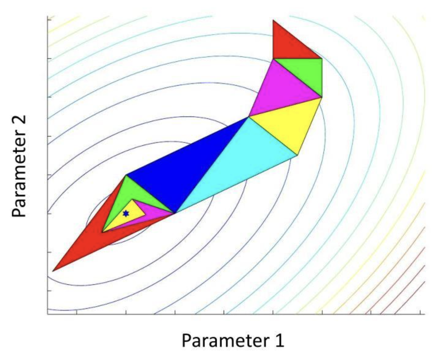
Source:
https://www.slideserve.com/nay/nelder-mead
Like gradient descent, Nelder–Mead is generally a local
optimizer.
Pitfalls and Takeaways
Common optimization traps
- Local
global minima: following downhill is not enough: a low valley
may not be the lowest valley
- Initial guesses: different
lead to different minima
- Step size (learning rate): a poor choice can cause
either slow or unstable convergence
- Dimensionality:
grid samples per coordinate require
evaluations!
Practical strategy: run the optimizer from
many starting configurations.
Avoiding Local Minima
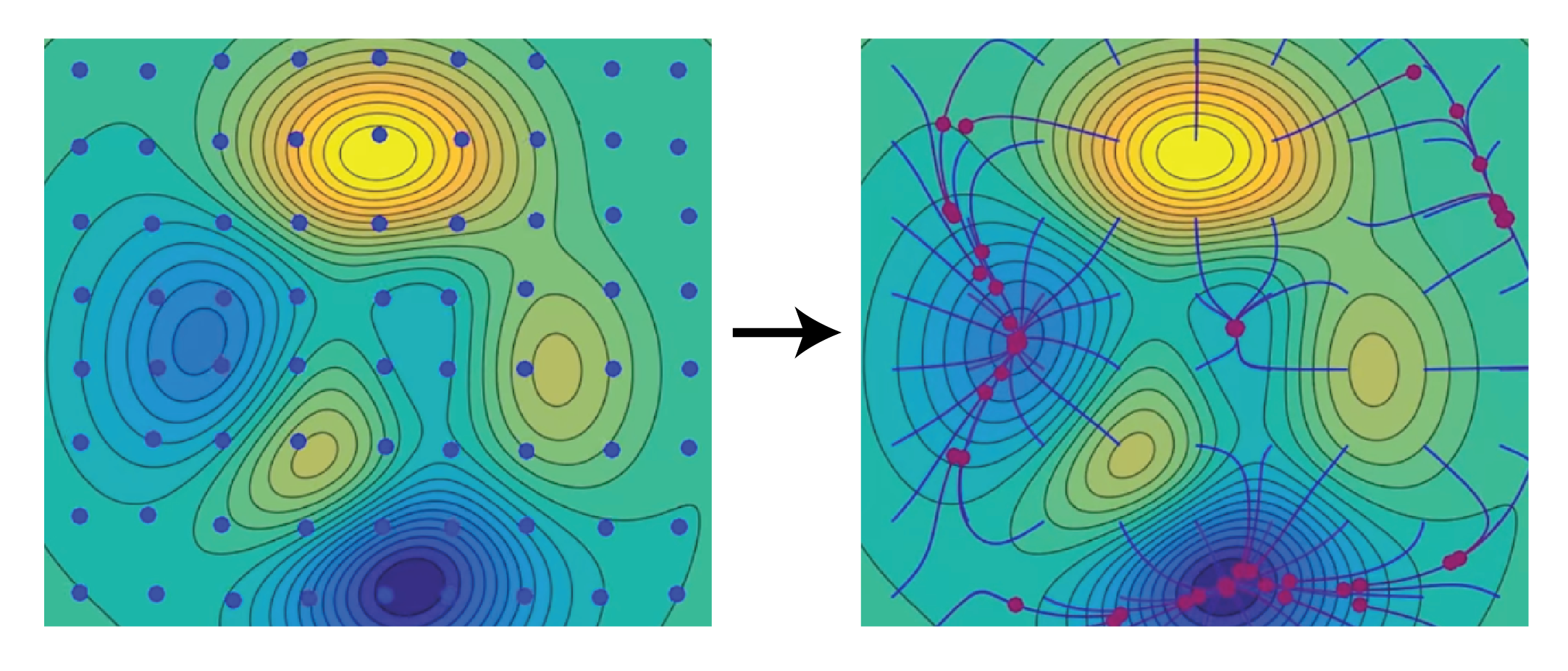
A downhill algorithm can get trapped
- Gradient descent is a local method
- The final answer can depend on the initial
guess
- A vanishing gradient does not guarantee the lowest
energy everywhere
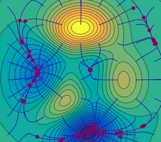
Source:
https://commons.wikimedia.org/wiki/File%3AGradient_Descent_in_2D.webm
Movie: Wikimedia
Commons: Gradient Descent in 2D
Question: How could we make the search more
reliable?
Multistart optimization: try many initial guesses
- Draw many starting configurations
- Run gradient descent from each
- Compare final energies and keep the lowest
Still no mathematical guarantee of a global
minimum.
AI-coding demo: automate multistart searches
Prompt a local AI model:
Starting from our four-bead protein
energy(theta1, theta2, ...) function located in
folding_model.py, write Python code that samples 100 random
initial angle configurations
,
runs gradient descent from each, and plots the trajectories on an energy
contour map. Highlight the lowest final energy. Do not change any
existing code, and write this Python code in a new file named
multistart_protein.py. Do not examine any
files other than folding_model.py and do
not leave the directory Lecture 14.
Verify its output:
- Does it actually launch 100 independent
searches?
- Are the angles treated as periodic?
- Are the final energies recalculated and compared?
- Does changing the random seed change which minima are
discovered?
Simulated annealing: sometimes go uphill!
Problem: strictly downhill steps cannot cross an
energy barrier.
New strategy: propose a random change and sometimes
accept an uphill move:
with
- Downhill moves: always accepted
- Uphill moves: accept with probability
Uphill moves are especially probable at high
temperature
,
but occur less frequently at low temperature.
Gradually lower
:
explore first, settle later.
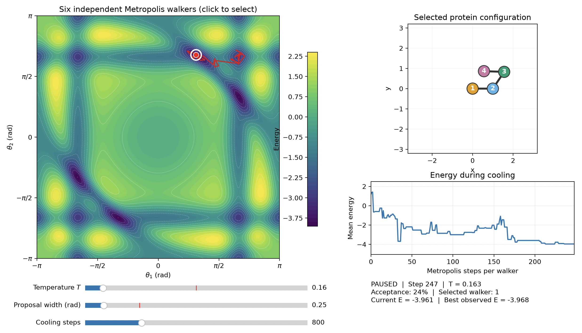
Demo: hot and cold searches
Same energy landscape, different temperatures:
- High
:
many uphill moves; explore broadly
- Low
:
uphill moves rare; become trapped more easily
- Cooling schedule: seek a compromise between
exploration and convergence
Connection to physics: thermal fluctuations and
Boltzmann weights.
Which method should we use?
| Gradient descent |
Yes (or finite differences) |
Simple, efficient local descent |
Initial-guess and step-size sensitivity |
| Multistart descent |
Yes (repeatedly) |
Explores multiple basins |
More computational work |
| Nelder–Mead |
No |
Uses function values only |
Can stagnate; local search |
| Simulated annealing |
No |
Can cross energy barriers |
Requires many evaluations and temperature tuning |
Takeaways
- Gradient descent moves against the local
gradient
- Learning rate controls convergence and
stability
- A local minimum is not necessarily the global
minimum
- Multistart and annealing improve
exploration in different ways
- The best method depends on the landscape and what we can
compute
Next: combinatorial optimization — when our choices
are discrete rather than continuous.