Logistics and Agenda

Homework 4 due Today Oct 19 at 11:59pm

Homework 5 due Monday Oct 26 at 11:59pm

Midterm 2

• Take-home posted Monday Oct 26
• In-class exam Monday Nov 2

Agenda

• This week:  Opimization in multiple dimensions
• Next week:  Advanced optimization, combinatoric optimization, machine learning

Today

Optimization in multiple dimensions

• Linear regression as an optimization problem
• Energy landscapes in two dimensions
• Four-bead protein folding model + AI demo
• Gradient descent optimization

Last time: optimizing a single variable

• Three-bead protein: one angle $\theta$
• Objective: minimize the energy $E(\theta)$
• Methods: bisection, Newton–Raphson, golden-section search

Today: what if the protein can bend at two joints $\theta_1, \theta_2$?

The multidimensional optimization problem

We choose a vector of adjustable parameters:

$$\vec{\theta}=(\theta_1,\theta_2,\ldots,\theta_d)$$

and try to minimize the objective function:

$$\boxed{\vec{\theta}_*=\arg\min_{\vec{\theta}} \ f(\vec{\theta})}$$

• One parameter: a curve
• Two parameters: a surface
• Many parameters: a high-dimensional landscape (hypersurface)

Reading a two-dimensional energy landscape

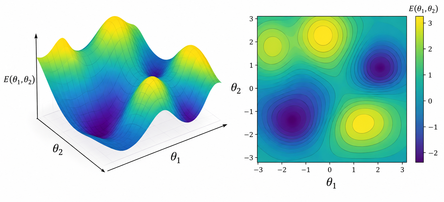
Source: generated with ChatGPT

• Valleys = low energy; hills = high energy
• Contour lines connect points with equal energy
• A local minimum may not be the global minimum

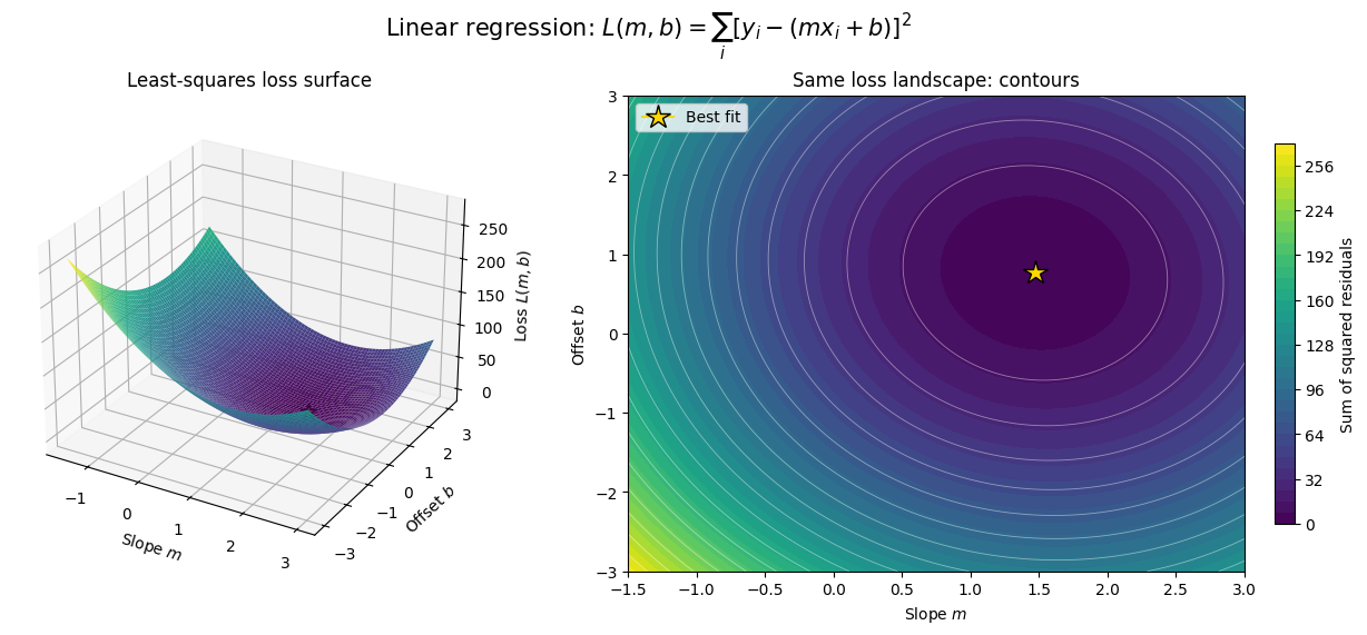
Linear regression as an optimization problem

Suppose we have $N$ fixed datapoints $(x_i,y_i)$ and want to fit a line:

$$\boxed{y_{\mathrm{fit}}(x)=mx+b}$$

Adjustable parameters: $\vec{\theta}=(m,b)$ = (slope, offset)

Linear regression as an optimization problem

Suppose we have $N$ fixed datapoints $(x_i,y_i)$ and want to fit a line:

$$\boxed{y_{\mathrm{fit}}(x)=mx+b}$$

Adjustable parameters: $\vec{\theta}=(m,b)$ = (slope, offset)

Objective function: sum of squared residuals

$$\boxed{\chi^2(m,b)=\sum_{i=1}^{N}[y_i-(mx_i+b)]^2}$$

Goal: Find $(m,b)$ that minimize $\chi^2$.

The Loss Landscape (objective function)

Every choice of $(m,b)$ corresponds to a point in the parameter space, with an associated cost $\chi^2(m,b)$.

Demo: python linear_fit_gui.py

Next: What happens when the landscape has multiple valleys?

Previously: Three beads, one angle

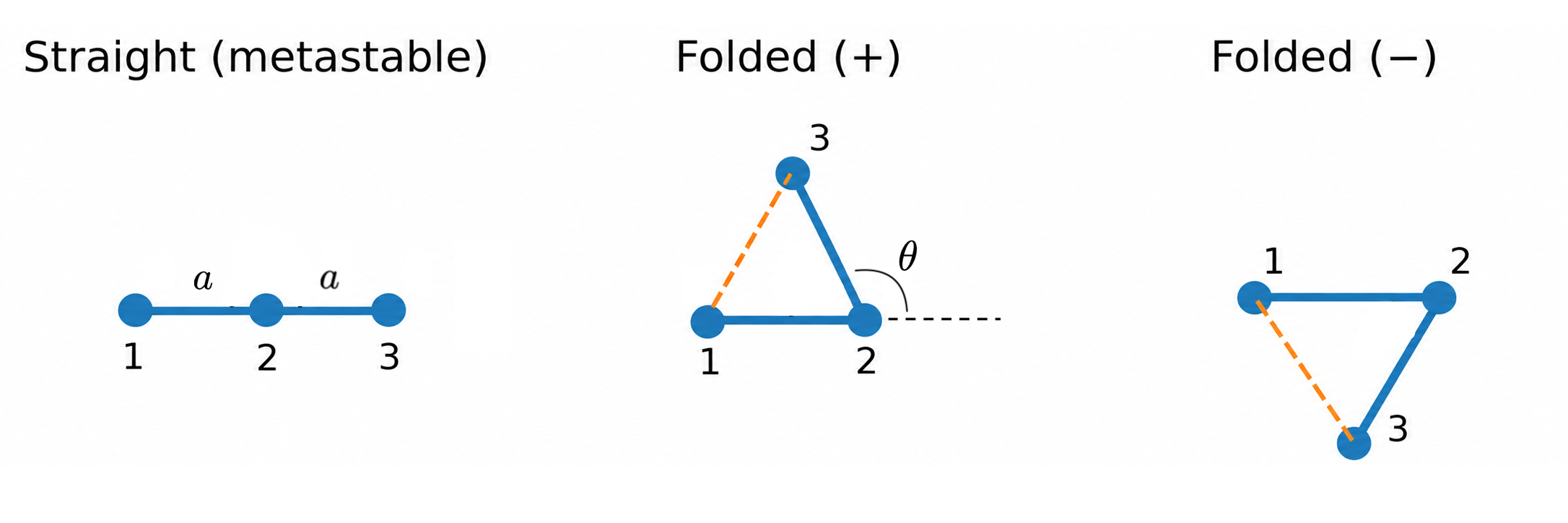
Source: generated with ChatGPT

Four beads, three links, two angles

Source: generated with ChatGPT

Three rigid links, two independent bending angles:

$$\vec\theta=(\theta_1,\theta_2), \qquad -\pi\le\theta_i\le\pi.$$

• Bending costs energy
• Non-neighboring beads attract
• The fold is now a point in a 2D parameter space $(\theta_1,\theta_2)$

Objective function: folding energy $E(\theta_1,\theta_2)$

$$\boxed{E(\theta_1,\theta_2)=\kappa(2-\cos\theta_1-\cos\theta_2) +V(r_{13})+V(r_{24})+V(r_{14})}$$

$$V(r)=-\epsilon\exp\!\left[-\frac{(r-r_0)^2}{2\sigma^2}\right]$$

Fixed parameters:

• $\kappa$: bending stiffness
• $\epsilon$: attractive interaction strength
• $r_0$: preferred separation
• $\sigma$: interaction range

Source: generated with ChatGPT

Adjustable parameters: $\theta_1, \theta_2$

The distances $r_{ij}$ are trig functions depending on $\theta_1, \theta_2$

AI Demo: translate physics into Python

Prompt a local model to generate:

bead_positions(theta1, theta2, a)
energy(theta1, theta2, a, kappa, epsilon, r0, sigma)

Specify the conventions:

• Bead 1 at $(0,0)$; first link along $+x$
• Subsequent link directions: $0$, $\theta_1$, $\theta_1+\theta_2$
• Attraction pairs: $(1,3)$, $(2,4)$, $(1,4)$
• Angles in radians
• energy function should be “vectorized” (i.e. allow $\theta_1,\theta_2$ to be arrays)

AI coding: test before trusting

Check geometry:

• At $(\theta_1,\theta_2)=(0,0)$: beads at $(0,0),(a,0),(2a,0),(3a,0)$
• Folding energy should agree with the displayed formula

Check numerically:

p = bead_positions(0, 0, 1.0)
assert np.allclose(p, [[0,0], [1,0], [2,0], [3,0]])
assert np.isfinite(energy(0., 0., 1., 1., 3., 1., .2))

Takeaway: AI can implement our physical model; we specify and validate it.

Exploring the folding landscape

Demo: folding_2d.py

1. Move the red marker: how does the chain fold?
2. Find a low-energy region: what does the chain look like?
3. Compare two distinct valleys: which fold has lower energy?
4. Change $\kappa$ or $\epsilon$: how does the landscape change?

Contrast with linear regression: this energy landscape can have several minima.

Challenge: How can a computer automatically find the valleys?

The gradient: which way is uphill?

For $E(\theta_1,\theta_2)$, define the gradient:

$$\boxed{\vec\nabla E=\begin{pmatrix} \partial E/\partial\theta_1\\[3pt] \partial E/\partial\theta_2 \end{pmatrix}}$$

• $\vec\nabla E$ points uphill (steepest local increase)
• $-\vec\nabla E$ points downhill (steepest local decrease)
• At a local minimum $\vec\nabla E=\vec 0$ (but so do maxima and saddle points!)

Source: generated with ChatGPT

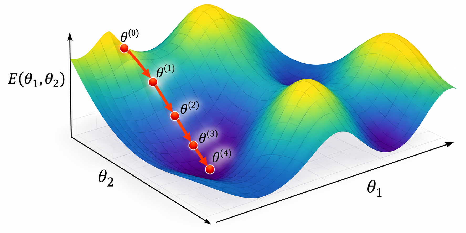
Gradient descent is an iterated map

Start with $\vec{\theta}_0$, then repeatedly step downhill:

$$\boxed{\vec\theta_{n+1}=\vec\theta_n-\eta \ \vec\nabla E(\vec\theta_n)}$$

• $\eta>0$: learning rate (step size)
• Evaluate gradient $\rightarrow$ step downhill $\rightarrow$ repeat
• Stop when energy / parameters stop changing appreciably

This is an iterated map, just like our earlier dynamical-systems examples.

Gradient descent in Python

Start with $\vec{\theta}_0$, then repeatedly step downhill:

$$\boxed{\vec\theta_{n+1}=\vec\theta_n-\eta \ \vec\nabla E(\vec\theta_n)}$$

import numpy as np

# grad_energy(theta) takes a length-2 array and returns the gradient (also length-2)

theta = np.array([1.0, -2.0])   # initial guess (radians)
eta = 0.05                      # learning rate
tol = 1e-6                      # convergence tolerance
max_steps = 1e4                 # maximum number of steps

grad = grad_energy(theta)
step = 0

while (np.linalg.norm(grad) > tol) & (step < max_steps):
    theta -= eta * grad
    grad = grad_energy(theta)
    step = step + 1

In practice: $\vec\nabla E$ may be derived analytically or approximated using finite differences.

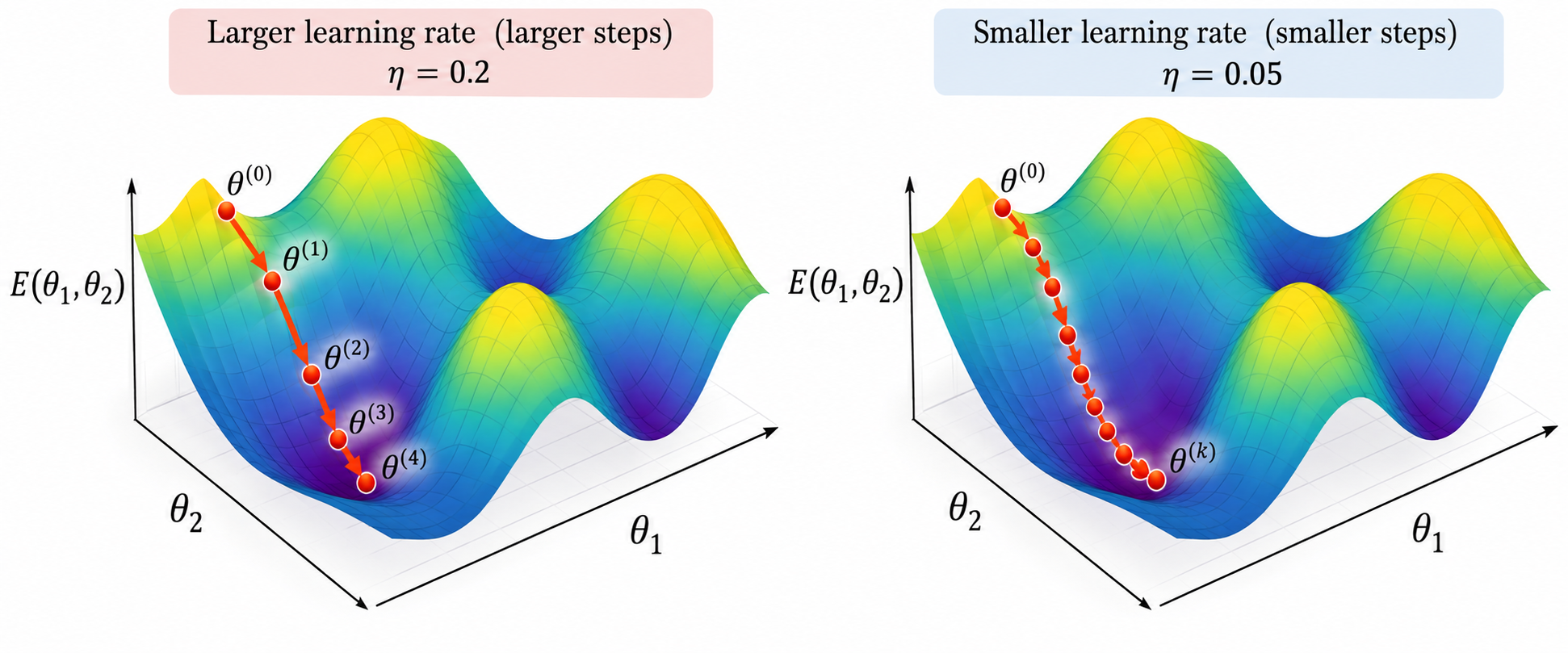
Demo: learning rate and starting guess

Demo: folding_gradient_descent.py

Source: generated with ChatGPT

• Small $\eta$: safe, but slow
• Large $\eta$: overshooting, oscillations, or divergence
• Different initial guesses: may converge to different minima

Question: How can we be confident we found the global minimum?

Common optimization traps

• Local $\ne$ global minima: following downhill is not enough: a low valley may not be the lowest valley
• Initial guesses: different $\vec{\theta_0}$ lead to different minima
• Step size: a poor choice can cause either slow or unstable convergence
• Coarse grids: may completely miss a narrow valley
• Dimensionality: $m$ grid samples per coordinate require $m^d$ evaluations!

Practical strategy: run the optimizer from many starting configurations.

Takeaways

The goal: minimize $E(\vec\theta)$ in a space with many possible configurations.

1. Visualize the landscape when you can
2. Use gradient descent to move downhill systematically
3. A converged answer is not necessarily the global minimum

AI-generated models and code

1. Prompts should be exhaustive and specific
2. Validate AI-generated numerical models against physical checks

Next time:

• What if we don’t have access to the gradient $\nabla E$?
• Deliberately move uphill to escape a local minimum?