Logistics and Agenda

Homework 4 due Monday Oct 19 at 11:59pm

Agenda

• This week:  Optimization in 1D
• Next week:  Opimization in multiple dimensions + combinatoric optimization

Today

• Optimization in one dimension
  • Local versus global minima
  • Revisit root-finding: bisection and Newton–Raphson
  • Golden-section search: minimize without derivatives
• Motivation: protein folding

What is optimization?

Many problems in physics ask us to find the best value of a variable $x$.

• Mechanics: find configurations of minimum potential energy.
• Data fitting: choose parameters that minimize $\chi^2$.
• Statistical mechanics: find energetically favorable states.

$$\boxed{x_* = \arg\min_{x\in[a,b]} f(x)}$$

Question: How can a computer find $x_*$ if we only know how to evaluate $f(x)$?

Local and global minima

A local minimum has lower energy than nearby configurations.

A global minimum has the lowest energy among all allowed configurations.

Why is it easy for a numerical method to mistake a local minimum for a global minimum?

Protein Folding: a grand challenge in physics & biology

Proteins are chains of amino acids that fold into complex three-dimensional structures.

Folding is driven by competing chemical interactions:

• Hydrogen bonding, electrostatic interactions, hydrophobic effects, van der Waals forces, etc.
• The resulting structure determines much of the protein’s biological function.

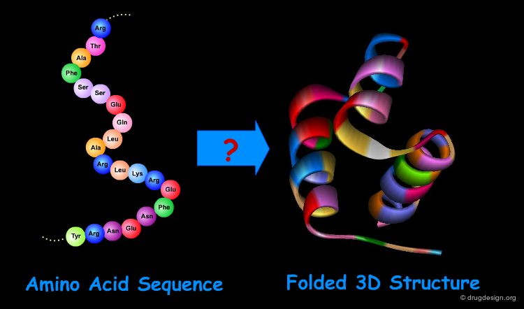
Source: https://www.drugdesign.org/chapters/protein-structure/

Protein Folding and Optimization

The challenge: Given a sequence of amino acids, what spatial structures can the protein adopt?

• Finding stable configurations is naturally an energy minimization problem.
• An enormous number of possible configurations!
• Each configuration is a local minimum (optimum) in an extremely complicated energy landscape.

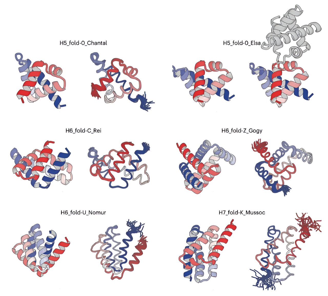
https://phys.org/news/2024-01-breakthrough-complicated-protein.html

Recent breakthrough: AlphaFold used AI to predict protein structures with remarkable accuracy, revolutionizing structural biology and contributing to the 2024 Nobel Prize in Chemistry.

Protein Folding and Optimization

Today:

• Build a dramatically simplified model that captures the competition between different physical interactions.
• Use numerical optimization to find the lowest-energy configurations.

Three beads, two links, one angle

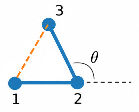
Consider three beads constrained to a 2D plane, connected by two rigid links of length $a$.

• Fix the position of bead 1 and the direction of the first link.
• The single degree of freedom is the bending angle $\theta\in[-\pi,\pi]$.
• The straight chain corresponds to $\theta=0$.

Source: generated with ChatGPT

Geometry: by the law of cosines,

$$r_{13}(\theta)=\sqrt{a^2+a^2+2a^2\cos\theta}=2a\cos(\theta/2).$$

Competing energies

We combine a bending penalty and an attractive bead-bead interaction:

$$\boxed{E(\theta)=\kappa(1-\cos\theta)-\epsilon\exp\!\left[-\frac{(2a\cos(\theta/2)-r_0)^2}{2\sigma^2}\right]}$$

• $\kappa$: bending stiffness (straight configurations favored)
• $\epsilon$: bead-bead interaction strength (negative energy near $r_{13}=r_0$)
• $r_0$: preferred bead-bead separation
• $\sigma$: width of the interaction well

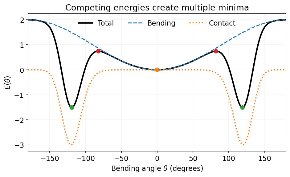
Default parameters: $a=1$, $\kappa=1$, $\epsilon=3$, $r_0=1$, $\sigma=0.2$.

Source: generated with ChatGPT

Competition: bending penalty versus attraction between beads

Demo: python code/folding_1d.py

Local and global minima

Default parameters: $a=1$, $\kappa=1$, $\epsilon=3$, $r_0=1$, $\sigma=0.2$.

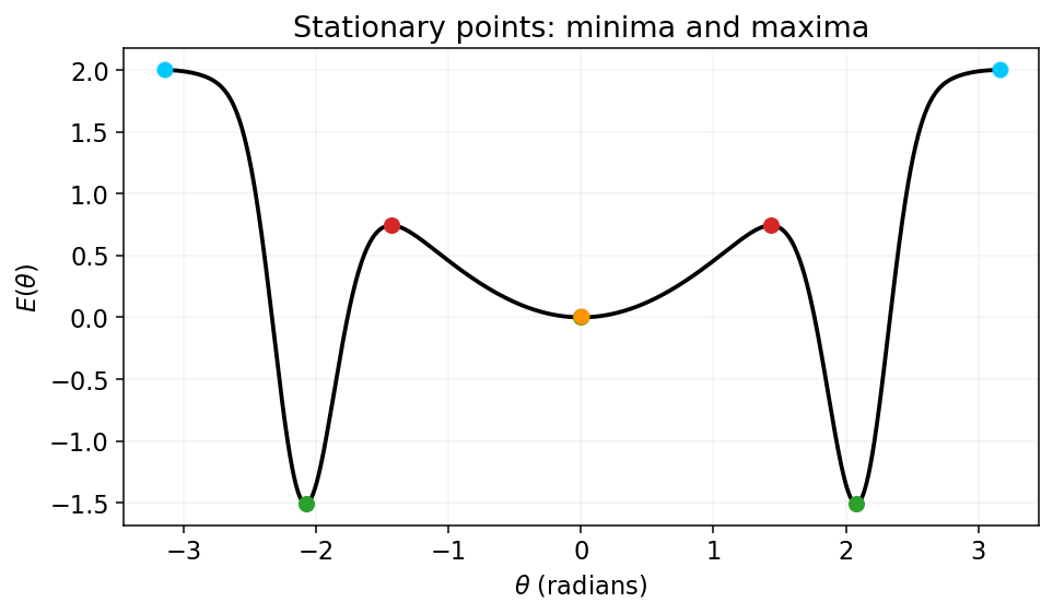
At the default parameters the landscape has three local minima:

• $\theta=0$: a metastable straight configuration, $E\approx 0$.
• $\theta\approx\pm2.078 \ \textrm{rad}$: two symmetry-related folded ground states, $E\approx-1.507$.
• Local maxima separate the minima at $\theta\approx\pm1.43 \ \textrm{rad}$.

Why two ground states? $E(-\theta)=E(\theta)$: mirror-related configurations have the same energy.

Connection to root finding

For an interior stationary point, we require

$$\boxed{\left.\frac{d E}{d \theta}\right\rvert_{\theta^*} \equiv E'(\theta_*)=0.}$$

We already know two methods for solving equations of the form $g(x)=0$:

• Bisection: find a sign change of $g=E'$ and repeatedly halve the bracket.
• Newton–Raphson: iterate $\theta_{n+1}=\theta_n- \frac{E'(\theta_n)}{E^{(2)}(\theta_n)} \quad \quad \quad \quad E^{(2)} \equiv \frac{d^2 E}{d \theta^2}$.

But beware: a stationary point could be a minimum or maximum.

$$E^{(2)}(\theta_*)>0:\ \text{local minimum},\qquad E^{(2)}(\theta_*)<0:\ \text{local maximum}.$$

Boundary minima also need to be checked separately.

Differentiating the folding energy

Let $r=r_{13}(\theta) = 2a\cos(\theta/2)$, where $\partial r / \partial \theta \equiv r'=-a\sin(\theta/2)$.

$$E'(\theta)=\kappa\sin\theta+\frac{\epsilon}{\sigma^2}(r-r_0)r'\exp\!\left[-\frac{(r-r_0)^2}{2\sigma^2}\right].$$

• Solving $E'(\theta)=0$ finds stationary configurations.
• In mechanics, this is a zero-torque condition (similar to zero forces).

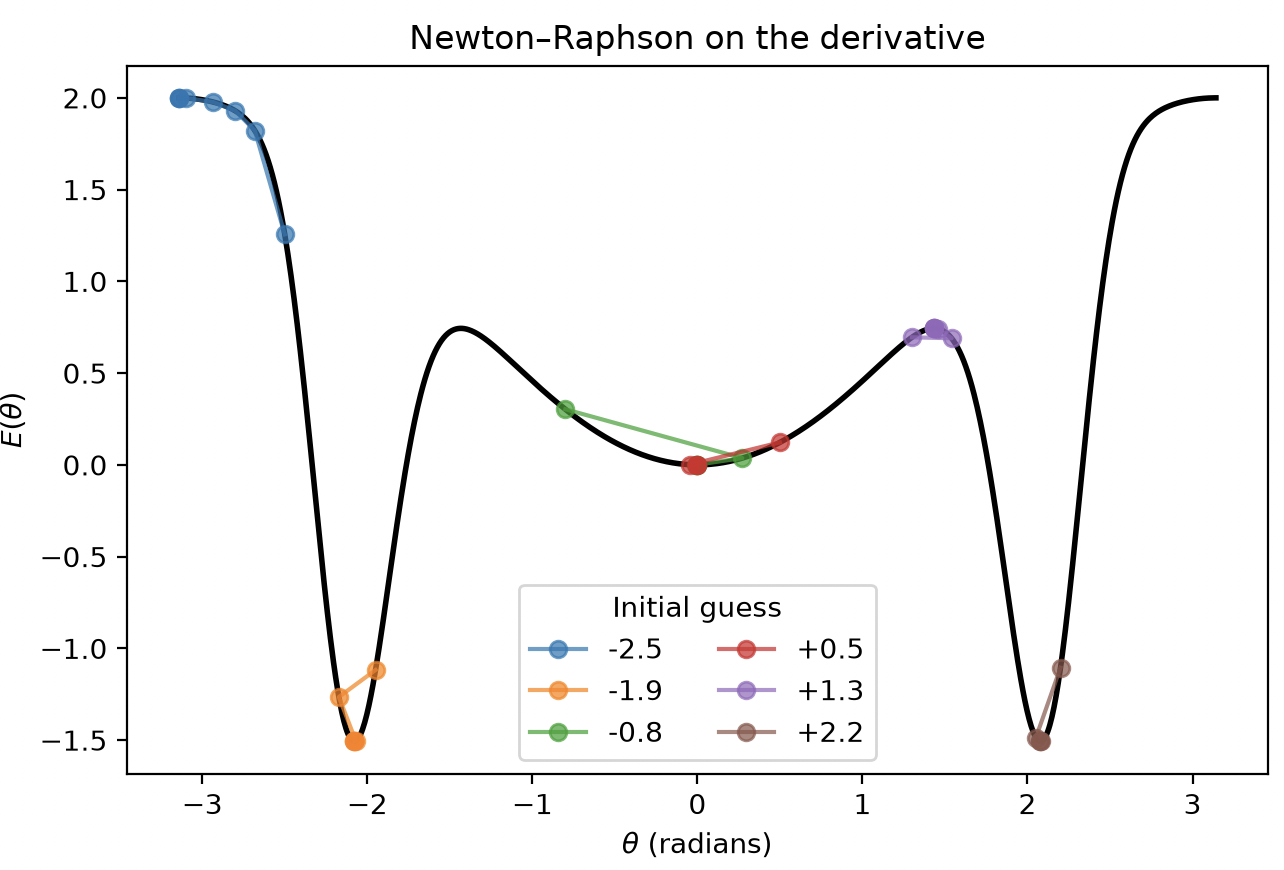
Demo: python code/root_vs_min.py

What can go wrong?

• Bisection on $E'$ may converge to a maximum.
• Newton–Raphson depends on its initial guess and may also find maxima.
  • To distinguish minima from maxima, we can compute $d^2 E / d \theta^2$ (concave vs convex)
  • We can also compare the energy $E$ itself
• A derivative root alone does not establish the global minimum.

In addition, in some situations the derivative $E'(\theta)$ may be unavailable or expensive to compute.

Question: Could we locate a minimum using only evaluations of $E$, without any derivatives?

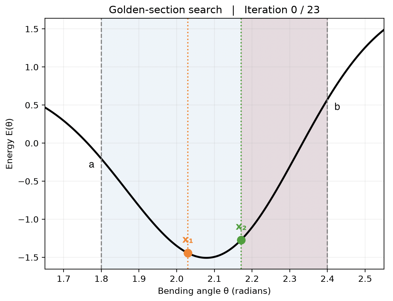
The idea behind golden-section search

Assume $f(x)$ is unimodal over an interval $[a,b]$: it decreases toward a single minimum and increases afterward.

Why the golden ratio?

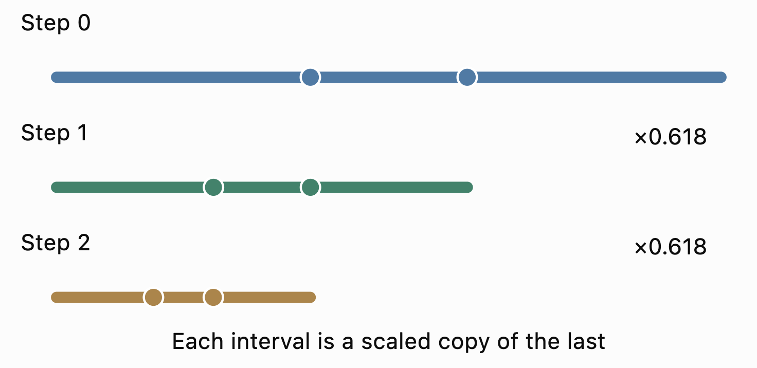
Choose points with the same fractional spacing at each iteration:

$$x_1=b-\frac{b-a}{\varphi},\qquad x_2=a+\frac{b-a}{\varphi},\qquad\varphi=\frac{1+\sqrt5}{2}.$$

The choice $\varphi^2=\varphi+1$ ensures that one interior point survives and its stored $f$-value can be reused.

• Two function evaluations to initialize.
• Only one new function evaluation per iteration.
• Bracket width shrinks by $1/\varphi\approx0.618$ each iteration.

Source: generated with ChatGPT

Demo: python code/golden_section_stepper.py

How many iterations?

After $n$ iterations, the bracket width is

$$L_n=\varphi^{-n}L_0.$$

To obtain $L_n\le\delta$:

$$\boxed{n\ge\frac{\ln(L_0/\delta)}{\ln\varphi}.}$$

Example: Starting from $L_0=0.6$, estimate the number of iterations needed for $\delta=10^{-6}$.

(Each iteration costs one new energy evaluation after initialization.)

Live coding — golden-section search

Task: Implement a function with the interface

def golden_section(f, a, b, tol=1e-6):
    """Find the minimum of a unimodal function on [a,b]."""

# Initialize interior points and their function values.

# Repeatedly discard the worse side, reusing one value.

# Return the midpoint of the final bracket.

$$x_1=b-\frac{b-a}{\varphi},\qquad x_2=a+\frac{b-a}{\varphi},\qquad\varphi=\frac{1+\sqrt5}{2}.$$

Validate using $f(x)=(x-2)^2+1$ over $[0,5]$

Reference solution and animation: python code/golden_section.py

Bracket choice matters

Surprise: On our symmetric example, golden-section search on the full interval converges near $\theta=0$, which is not the global minimum.

How could we search more globally?

A simple strategy in one dimension:

1. Evaluate the energy on a coarse grid.
2. Identify promising intervals containing local minima.
3. Run a local optimizer in each interval.
4. Compare the resulting energies (and check the endpoints).

This strategy helps explore a multimodal landscape but does not guarantee finding an arbitrarily narrow, hidden minimum.

Challenge: What becomes harder when there are two or three independent bending angles?

Review

• Optimization asks us to minimize an objective function.
• Root-finding can locate stationary points when derivatives are available; not every stationary point is a minimum.
• Golden-section search is derivative-free, inexpensive, and reliable for a unimodal bracket.
• Efficient local minimization is different from finding the global minimum.

Next lecture: four- and five-bead chains, energy landscapes in several dimensions, and gradient descent as an iterated map.