Agenda

Today

• Review 2D NumPy arrays and indexing
• Simulate a virus outbreak on a lattice
• Optimize a vaccination policy
• Simulate a forest fire and discover percolation
• Optimize tree removal to prevent fire spread

Main ideas:

• A simulation predicts what happens for a choice of parameters.
• Optimization selects parameters to achieve a desired outcome.

Simulation and Optimization

A simulation takes a model and parameters and predicts an outcome.

$$\text{parameters }\theta\ \longrightarrow\ \text{simulation}\ \longrightarrow\ \text{outcome}.$$

An objective function assigns a numerical cost to that outcome:

$$J(\theta)=\text{cost associated with the outcome of parameters }\theta.$$

Optimization means finding the parameters with the lowest cost:

$$\boxed{\theta^*=\arg\min_{\theta}J(\theta).}$$

Examples:

• Simulating the path of a rocket from earth to mars
• Simulating the behavior of the stock market
• Simulating the flow of traffic and traffic lights

Simulation and Optimization

This builds on our iterated maps from last week:

• Simple rules
• Iteration
• Complex behavior

But this time we’ll be adding a few new ingredients

• randomness
• objective functions
• modification of parameters to optimize the objective function

Today: two spatial simulations, two objective functions.

Review: Indexing a 2D array

A 2D NumPy array uses row, column indexing:

A = np.array([
    [0.3, 0.8, 0.1, 0.6, 0.9],
    [0.7, 0.2, 0.5, 0.4, 0.1],
    [0.9, 0.6, 0.3, 0.8, 0.2],
    [0.4, 0.1, 0.7, 0.5, 0.6]
])

print(A[2, 0])       # one element

print(A[1, :])       # one row
print(A[:, 2])       # one column

print(A[1:3, 2:4])   # subarray (what size?)

print(A[4,4])
print(A[:,5])

Predict before running: What shape and value(s) does each expression return?

Key distinction: A[i, j] selects a cell; A[i, :] and A[:, j] select a row or column.

A population on a 2D grid

Divide a region into an $L\times L$ lattice. Each site contains either zero or one person.

Let $n_{ij}\in\{0,1\}$ indicate whether site $(i,j)$ is occupied:

$$n_{ij}\sim\operatorname{Bernoulli}(p),$$

where $p$ is the probability a site is occupied (and the average number of people per site).

import numpy as np

rng = np.random.default_rng(4)

L = 50
p = 0.65
occupied = rng.random((L, L)) < p

A spatial SIR model

Use one integer-valued array state to describe each site:

• 0: empty
• 1: susceptible
• 2: infected
• 3: recovered
• 4: vaccinated

An occupied site holds exactly one person, whose state changes over time; an empty site remains empty.

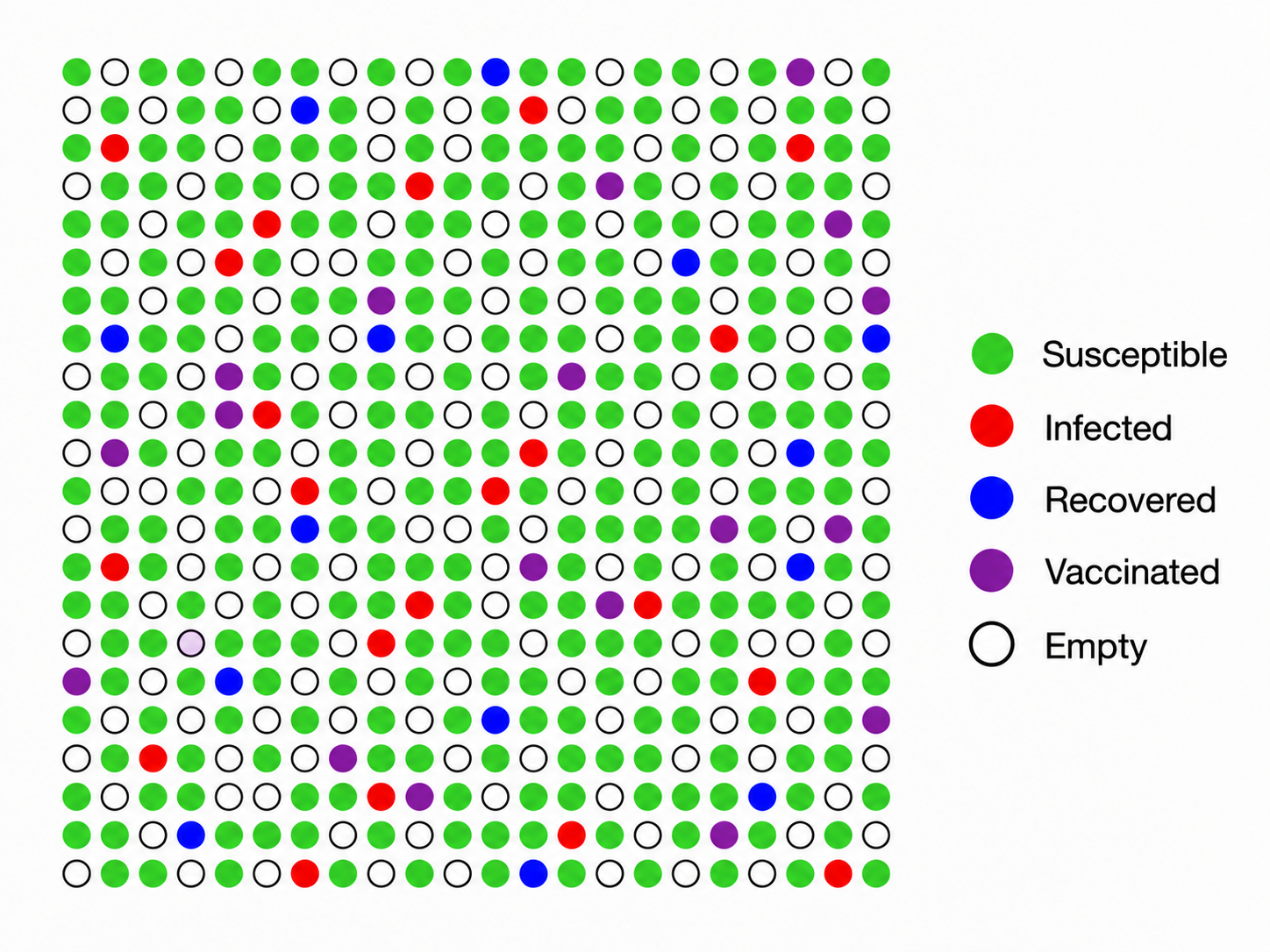
Source: generated with ChatGPT

Initially, vaccinate a fraction $v$ of occupied sites, then seed a few infections among the remaining susceptible people.

A spatial SIR model

Control parameter:

• Fraction of population $v$ that is vaccinated

Other parameters: (not in our control)

• Population density $p$
• Number of initial infections (5)
• Infection probability $\beta$
• Recovery probability $\gamma$

Transmission and recovery

Let $k_{ij}$ count infected people on the four nearest-neighbor sites. Since there is at most one person per site, $0\leq k_{ij}\leq4$.

A susceptible person becomes infected with probability

$$P_{ij}=1-(1-\beta)^{k_{ij}},$$

where $\beta$ is the transmission probability per infected neighbor per step.

Each infected person recovers with probability $\gamma$ per step.

Update rules:

• susceptible $\to$ infected with probability $P_{ij}$
• infected $\to$ recovered with probability $\gamma$
• Empty, recovered, and vaccinated sites do not change.

Determine all transitions from the old state, then apply them simultaneously.

Review: Count nearest neighbors with slicing

How can we add the four neighboring infected counts without writing a loop over every grid cell?

infected = (state == 2)         # Boolean array

k = np.zeros_like(state, dtype=int)

k[1:, :]  += infected[:-1, :]  # neighbor above
k[:-1, :] += infected[1:, :]   # neighbor below
k[:, 1:]  += infected[:, :-1]  # neighbor to the left
k[:, :-1] += infected[:, 1:]   # neighbor to the right

Check: Why do the two slices on each line have the same shape?

Boundary condition: No wraparound at the edges.

Boolean masks and vectorized updates

Rather than updating sites one at a time, use Boolean masks and vectorized operations.

susceptible = (state == 1)
infected = (state == 2)
P = 1 - (1 - beta)**k

new_infections = susceptible & (rng.random(state.shape) < P)
new_recoveries = infected & (rng.random(state.shape) < gamma)

state[new_infections] = 2
state[new_recoveries] = 3

Demo: Simulate an outbreak

Hold $\beta$ and $\gamma$ fixed. Compare different site-occupancy probabilities $p$ and vaccination fractions $v$.

• Plot infected people versus time: $I_{\mathrm{tot}}(t)=\sum_{ij} I_{ij}(t)$.
• Animate the spatial distribution of infection.
• Compare the final number ever infected.

Predict: What happens when we increase $p$? What happens when we increase $v$?

Optimization 1: Vaccination costs versus infection costs

Vaccination prevents infections, but vaccination itself has a cost.

Let $C(v)$ be the cumulative number of people infected over the outbreak, including initial infections. Let $N$ be the total population and $N_V(v)$ the number vaccinated.

Define the objective

$$\boxed{J_{\mathrm{virus}}(v)=\mathbb{E}\!\left[\frac{C(v)}{N}\right]+\lambda_v\,\mathbb{E}\!\left[\frac{N_V(v)}{N}\right].}$$

• First term: expected infected fraction
• Second term: vaccination cost, weighted by $\lambda_v$
• Choose $0\leq v\leq1$ to minimize $J_{\mathrm{virus}}(v)$

Why not just minimize the number of infections?

Optimize by scanning parameters

Evaluate the objective for a set of candidate vaccination fractions.

v_values = np.linspace(0, 1, 21)
J_values = np.array([virus_objective(v)[2] for v in v_values])

best_index = np.argmin(J_values)

Here virus_objective(v) estimates the expected cost by averaging over many independent outbreaks.

Discussion: How would the optimum change if vaccination became more expensive ($\lambda_v$ increased)?

A simpler spreading model

Represent a forest by a Boolean occupancy array:

$$A_{ij}=\begin{cases}1 & \text{tree},\\0 & \text{empty} .\end{cases}$$

Each site independently contains a tree with probability $p$.

p = 0.65
forest = rng.random((L, L)) < p

Fire begins on occupied sites along the left edge.

At every step, burning trees ignite all adjacent unburned trees, and then become burned.

Important: Fire spread is deterministic once the forest is generated.

Demo: Vary the tree density

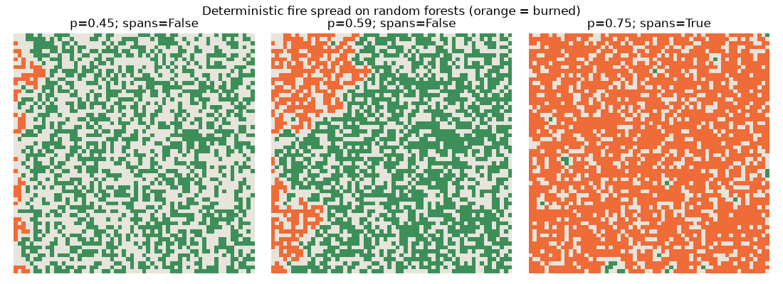
Try $p=0.45$, $p=0.59$, and $p=0.75$.

• Does the fire reach the right edge?
• How many trees burn?
• Do repeated random forests give the same outcome?

Even though fire propagation is deterministic, the forest itself is random.

Percolation: A connectivity transition

A connected cluster consists of trees joined by nearest-neighbor steps.

In this model, the trees that eventually burn are the connected clusters that are connected to the ignition boundary.

Therefore,

$$\Pr(\text{fire reaches right edge}) =\Pr(\text{a left-right connected cluster exists}).$$

For independent site percolation on a large square lattice,

$$\boxed{p_c\simeq0.5927.}$$

Below $p_c$, spanning is unlikely on a large lattice; above $p_c$, it is likely.

Estimating the spanning probability

A single random forest answers yes or no. Many trials estimate a probability.

$$P_{\text{span}}(p)\approx\frac{\text{number of trials that span}}{\text{total number of trials}}.$$

p_values = np.linspace(0.35, 0.85, 21)
probabilities = [
    np.mean([fire_spans(p) for _ in range(100)])
    for p in p_values
]

Question: Why is the transition smooth for a finite grid rather than perfectly sharp at $p_c$?

Optimization 2: Preventing forest fires

Suppose we start with a dense forest of tree density $p_0$.

Remove a fraction $q$ of the existing trees at random. The remaining density is

$$p=p_0(1-q).$$

Removing trees costs money; letting the fire reach the opposite side causes damage.

Define

$$\boxed{J_{\text{fire}}(q)=P_{\text{span}}\big(p_0(1-q)\big)+\lambda_f q.}$$

• First term: risk of a crossing fire
• Second term: cost of clearing a fraction $q$ of trees
• Choose $0\leq q\leq1$ to minimize $J_{\text{fire}}(q)$

Predict the optimal removal fraction $q$

From the percolation threshold,

$$p_0(1-q_c)=p_c.$$

Thus,

$$\boxed{q_c=1-\frac{p_c}{p_0}.}$$

For $p_0=0.80$,

$$q_c\approx1-\frac{0.5927}{0.80}\approx0.26.$$

Prediction: Removing roughly $26\%$ of the existing trees moves the remaining forest through the percolation threshold.

Does that guarantee the minimum of $J_{\text{fire}}$ occurs at $q_c$? No—the answer depends on $\lambda_f$ and finite-size effects.

Demo: Minimize fire risk and removal cost

For each value of $q$:

1. Generate many forests with density $p=p_0(1-q)$.
2. Compute the fraction of fires that reach the far edge.
3. Add the removal cost $\lambda_f q$.
4. Plot $J_{\text{fire}}(q)$ and locate its minimum.

q_values = np.linspace(0, 0.6, 31)
J_values = np.array([fire_objective(q) for q in q_values])
q_best = q_values[np.argmin(J_values)]

Review

Virus outbreak

• Random population: $n_{ij}\sim\operatorname{Bernoulli}(p)$
• Stochastic infection and recovery
• Choose vaccination fraction $v$ to balance health and intervention costs

Forest fire

• Random occupancy: $A_{ij}\sim\operatorname{Bernoulli}(p)$
• Deterministic spreading on a fixed forest
• Choose tree-removal fraction $q$ to balance fire risk and clearing costs

Looking ahead: How do we find the best parameters?

Today, we evaluated the objective on a grid of candidate parameter values:

$$J(\theta_1),J(\theta_2),\ldots,J(\theta_m).$$

But what if there are many parameters, or each simulation is expensive?

• Can we search more efficiently than testing every possibility?
• How do noise, local minima, and constraints affect optimization?
• How can we use derivatives to guide the search?

Next: Numerical optimization algorithms.