Agenda

Today

• Iterated maps, fractals, and chaos

Big idea:  Simple deterministic rules can generate surprisingly complicated behavior when repeated over and over.

Three examples:

• Newton-Raphson root-finding as a dynamical system
• Mandelbrot Set and fractals
• Logistic Map and population growth

Iterated maps

An iterated map repeatedly applies the same rule:

$$x_{n+1} = F(x_n).$$

Starting from an initial value $x_0$, we generate an orbit

$$x_0,\quad x_1,\quad x_2,\quad x_3,\quad \ldots$$

Computationally:

x = x0

for n in range(N):
    x = F(x)

Today we will ask:

What happens after we apply $F$ over and over again?

A simple linear example

Consider the iterated linear map

$$F(x)=a x.$$

Starting from $x_0$, the orbit is $x_0, \quad a x_0, \quad a^2 x_0, \quad \ldots, \quad$ The exact solution is therefore

$$x_n=a^n x_0.$$

Different values of $a$ give qualitatively different long-time behavior. Starting from $x_0=1$:

Fixed points

A fixed point $x^*$ satisfies

$$F(x^*) = x^*$$

meaning that the orbit is constant for all time.

• For $F(x) = a x$ the fixed point is $x^* = 0$.

• For $F(x) = x^2$ there are two fixed points: $x^* = 0,1$.

If the orbit approaches $x^*$,

$$x_n \rightarrow x^*,$$

then $x^*$ is a stable (attractive) fixed point.

If the orbit diverges from the fixed point, it is repulsive.

Stability of a fixed point

Suppose we start close to a fixed point:

$$x_n = x^* + \delta_n.$$

For small $\delta_n$ we may Taylor expand:

$$\begin{aligned} F(x^*+\delta_n) &\approx F(x^*) + F'(x^*)\delta_n \\ &= x^* + \delta_{n+1} \end{aligned}$$

Since $F(x^*)=x^*$,

$$\delta_{n+1} \approx F'(x^*)\delta_n.$$

Therefore:

$$|F'(x^*)| < 1 \quad \Rightarrow \quad \text{stable}$$

$$|F'(x^*)| > 1 \quad \Rightarrow \quad \text{unstable}$$

Stability in the linear example

$$F(x)=a x.$$

Since

$$F'(x)=a,$$

the fixed point $x^*=0$ is stable when

$$|a|<1, \quad \quad \quad \quad \quad \quad \quad a = \frac{1}{2}: \quad \quad 1, \quad \frac12, \quad \frac14, \quad \frac18, \quad \cdots, \quad 0$$

and unstable when

$$|a|>1, \quad \quad \quad \quad \quad \quad a = 2: \quad \quad 1, \quad 2, \quad 4, \quad 8, \quad \cdots$$

and marginal when

$$|a|=1, \quad \quad \quad \quad \quad \quad a = -1: \quad \quad 1, \quad -1, \quad 1, \quad -1, \quad \cdots$$

A nonlinear example

For the linear example, it doesn’t matter what initial condition $x_0$ you choose. The iterated map is globally stable or unstable depending on the parameter $a$.

Things get more interesting for nonlinear maps. Consider

$$F(x) = x^2$$

The fixed points $x^*$ satisfy $x^* = (x^*)^2$, so we have two fixed points

$$x^* = 0, \quad 1$$

Are these fixed points stable or unstable? Use the derivative criterion $|F'(x)| < 1$.

$$F'(x) = 2 x$$

• At $x^* = 0$ we have a stable fixed point since $|F'(0)| = 0$.

• At $x^* = 1$ we have an unstable fixed point since $|F'(1)| = 2$.

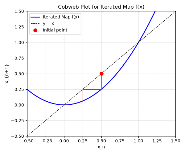
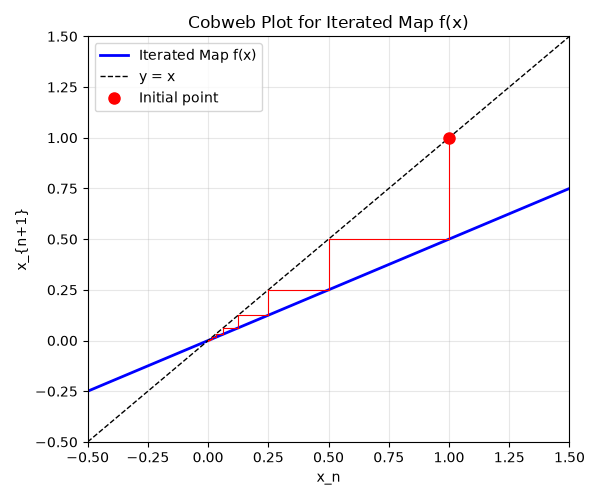
Cobweb plots

We can find and study fixed points visually in the $x-y$ plane.

To do this, let’s split each step of the iterated map onto two pieces:

$$y = F(x) \quad \quad \quad \quad x = y$$

Fixed points satisfy $F(x^*) = x^*$. This can be viewed as the intersection of these two functions.

And long-term behavior can be viewed as “ping-ponging” back and forth between these two functions.

$F(x) = a x, a = 1/2$

$F(x) = x^2$

Newton-Raphson revisited

Newton-Raphson finds roots of

$$f(x)=0$$

using

$$x_{n+1} = x_n-\frac{f(x_n)}{f'(x_n)}.$$

Define the Newton map

$$F(x)=x-\frac{f(x)}{f'(x)}.$$

Then Newton-Raphson is simply

$$x_{n+1}=F(x_n).$$

Every root $x^*$ of $f$ is a fixed point:

$$f(x^*)=0 \quad\Rightarrow\quad F(x^*)=x^*.$$

Root-finding in the complex plane

Consider finding roots of

$$f(z)=z^3-1.$$

The roots are complex

$$z_1=1,$$

$$z_2=e^{2\pi i/3}, \qquad z_3=e^{4\pi i/3}.$$

Q: can we find these roots via Newton-Raphson? From the previous slide we obtain the Newton map:

$$F(z) = z-\frac{f(z)}{f'(z)} = z-\frac{z^3-1}{3z^2}$$

or

$$F(z) = \frac{2}{3}z+\frac{1}{3z^2}$$

Clearly the roots $z_1,z_2,z_3$ are fixed points of this map.

Question:  Given an initial guess $z_0$, which root does Newton-Raphson find?

Demo: Newton-Raphson in the complex plane

For each starting point

$$z_0=x+iy,$$

run Newton-Raphson until it converges.

Color the starting point according to the root it reaches.

Algorithm:

1. Make a grid of initial conditions $z_0$.
2. Iterate Newton-Raphson at every point.
3. Determine which root each point approaches.
4. Assign each root a different color.

Basins of attraction

Each root has a basin of attraction:

$$B_i = \left\{ z_0: z_n \rightarrow z_i \right\}.$$

Points in the same basin converge to the same root.

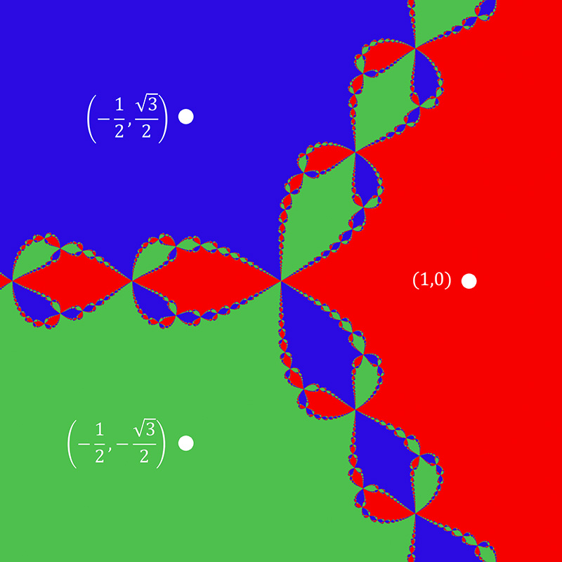
Source: https://paulbourke.net/fractals/newtonraphson/

What happens near the boundary?

Points that begin very close together can converge to different roots.

Zooming into the boundary reveals new structure at smaller and smaller scales.

This is our first example of a fractal.

A useful working definition:

A fractal has nontrivial structure that persists as we examine it at finer scales.

A lesson from Newton-Raphson

Newton-Raphson is:

• Deterministic
• Defined by a simple formula $F(z) = \frac{2}{3}z+\frac{1}{3z^2}$
• Easy to implement

Yet its global behavior can be extremely complicated.

The complexity does not come from randomness.

It comes from repeatedly applying a nonlinear map.

Simple rule + iteration $\rightarrow$ complex structure

An even simpler map

Consider

$$\boxed{ z_{n+1}=z_n^2+c }$$

with

$$z_0=0$$

and $c = a+i b$ a complex number.

For each complex value of $c$, generate the orbit

$$0,\quad c,\quad c^2+c,\quad \ldots$$

Then ask:

Does the orbit remain bounded, or does it escape to infinity?

Demo: iterate $z_{n+1}=z_n^2+c$

For one value of $c$:

z = 0

for n in range(N):
    z = z*z + c

    if abs(z) > 2:
        break

Try several choices of $c$.

Observe:

• Some orbits escape rapidly.
• Some settle into simple behavior.
• Some remain bounded but behave in complicated ways.

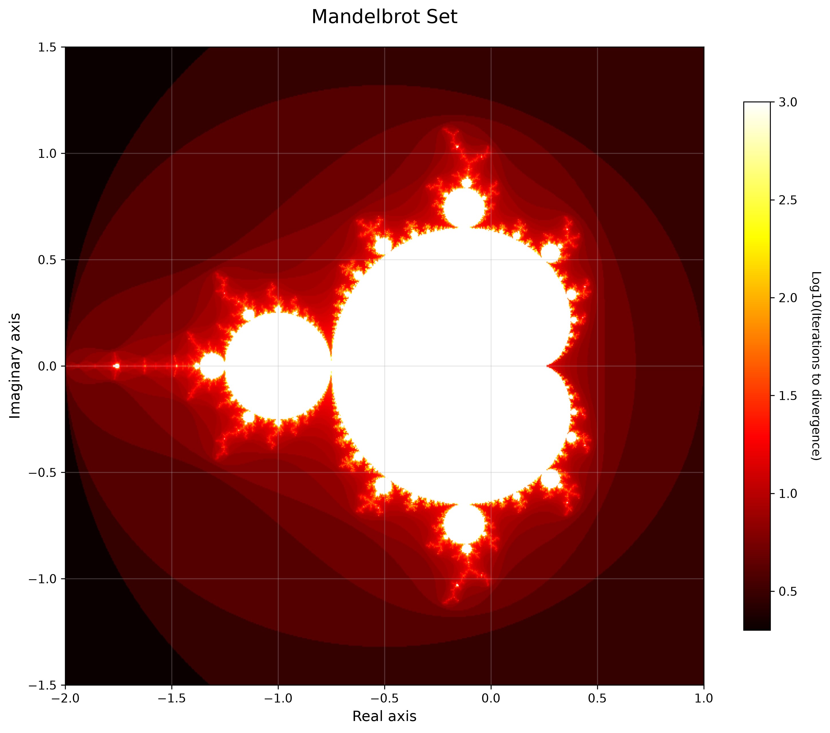
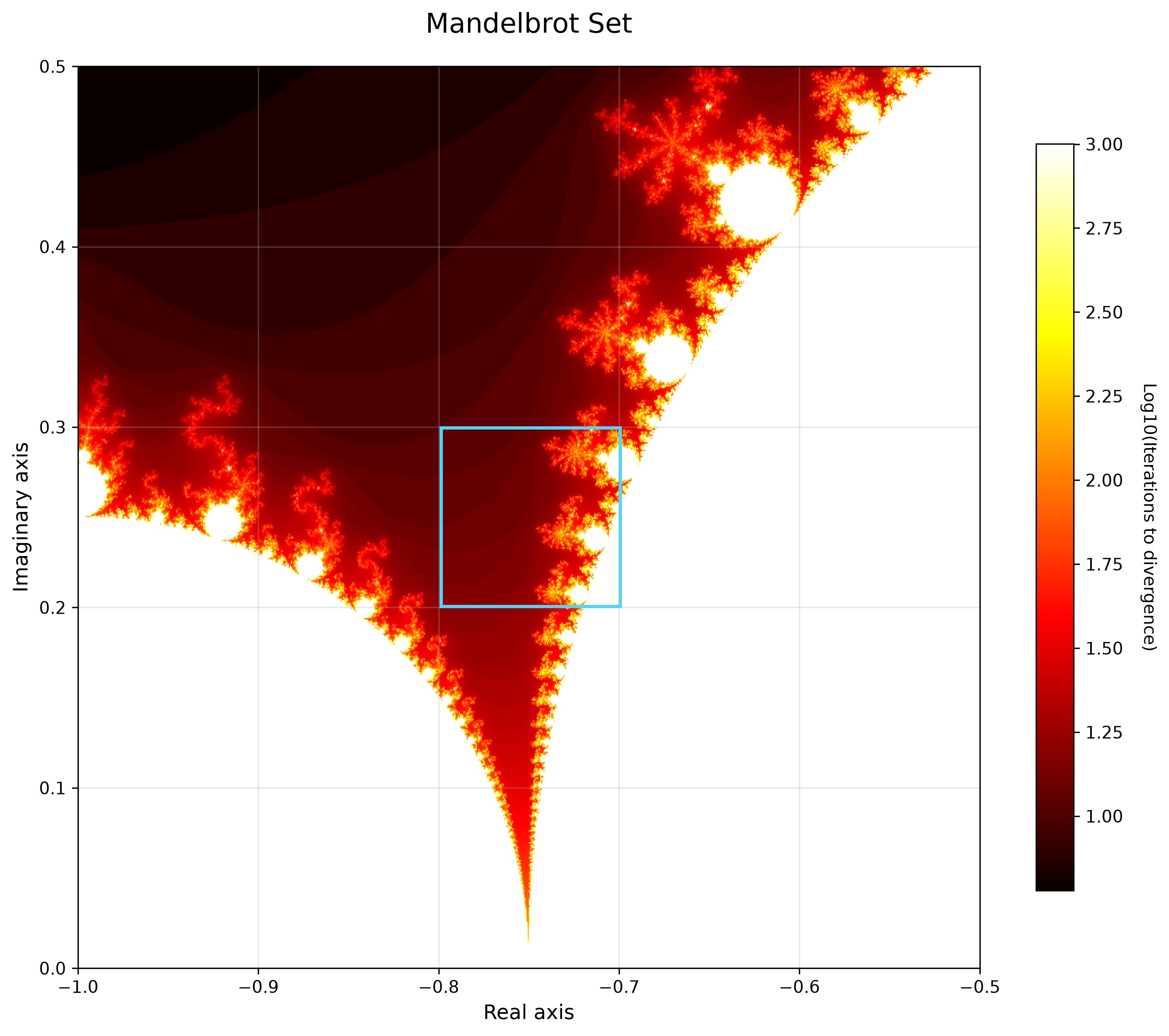
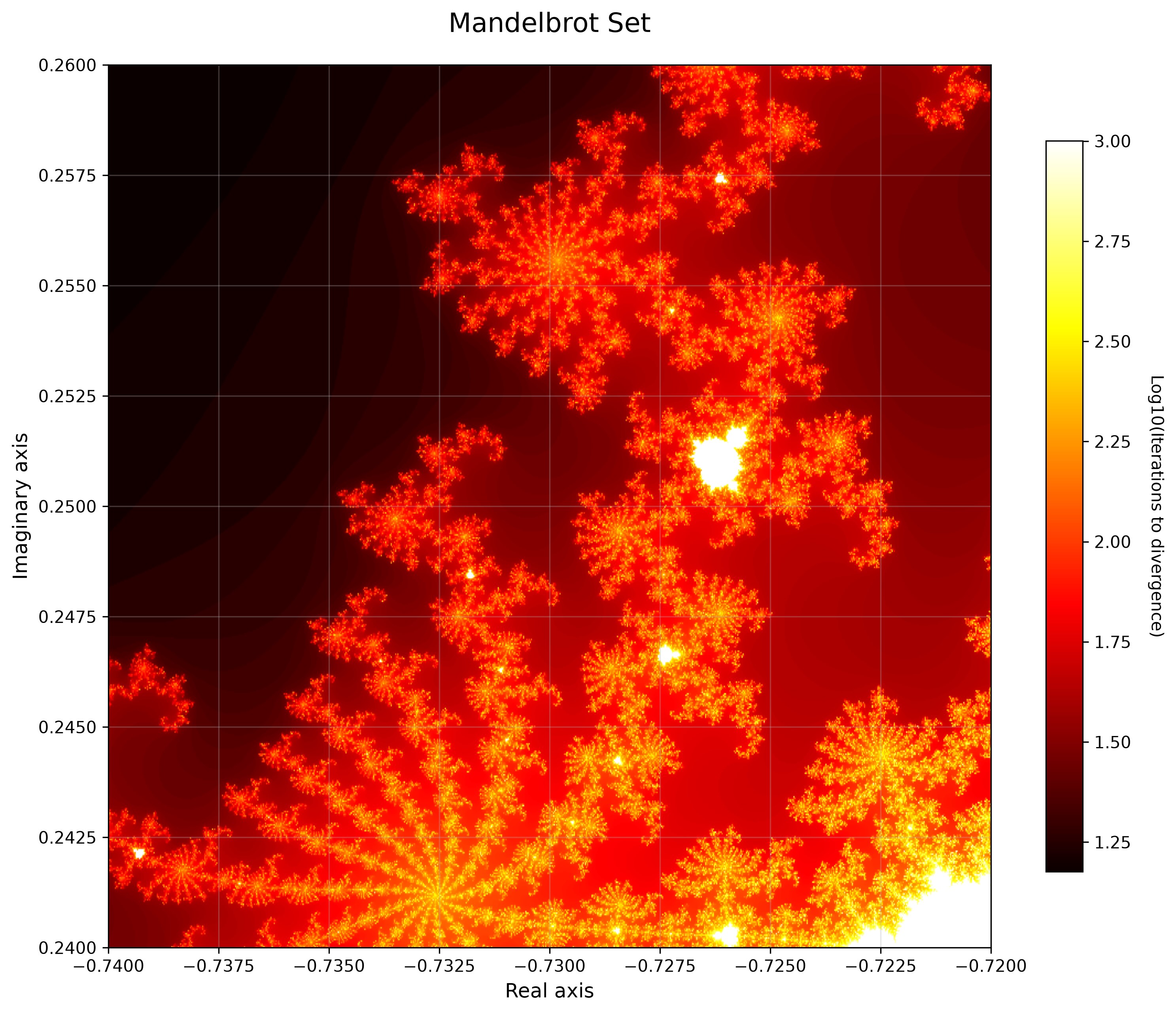
The Mandelbrot set

The Mandelbrot set is the collection of parameters $c$ for which the orbit remains bounded:

$$\mathcal{M} = \left\{ c\in\mathbb{C}: z_{n+1}=z_n^2+c,\; z_0=0 \text{ remains bounded} \right\}.$$

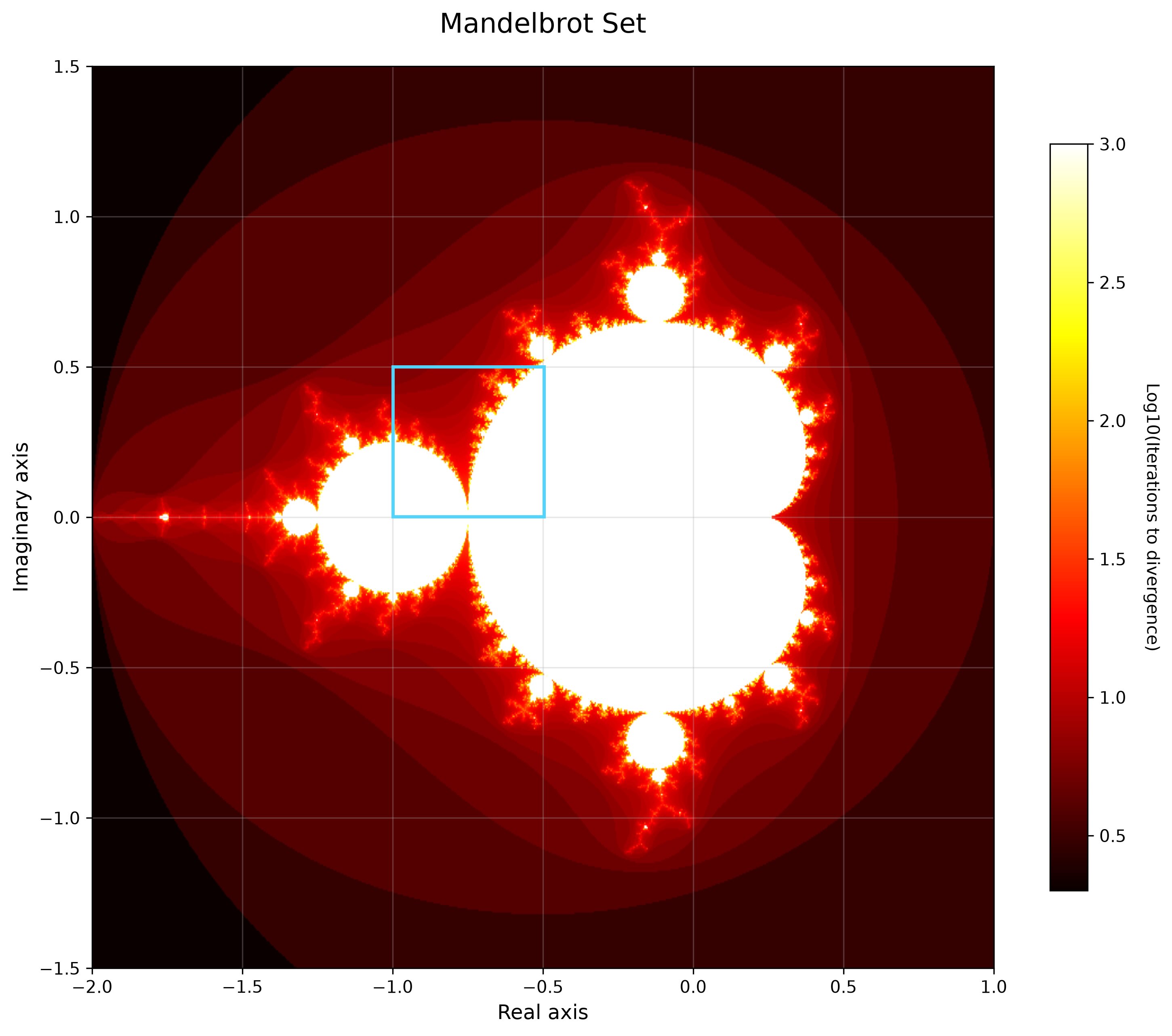
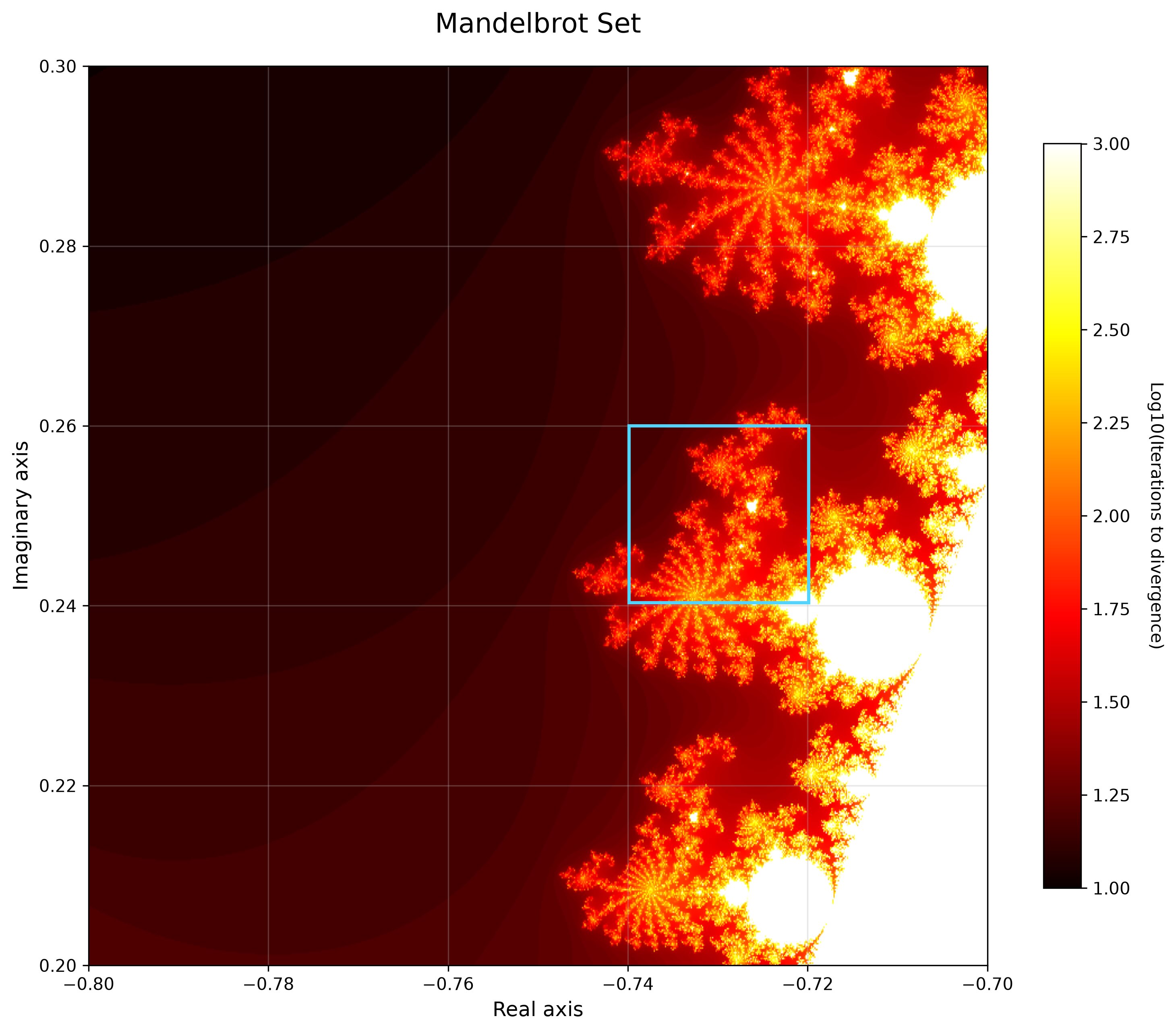
The Mandelbrot set, fractals, and self-similarity

Newton fractal vs. Mandelbrot set

Both reveal complicated structure by running a simple algorithm many times.

Computational strategy:  Scan over many inputs, iterate, then classify the long-time behavior.

Population growth

Suppose $x_n$ is the population during generation $n$, normalized so that

$$0\leq x_n\leq 1.$$

With unlimited resources, we might expect

$$x_{n+1}=r x_n.$$

But unlimited exponential growth is unrealistic.

Growth should slow when the population becomes large.

The logistic map

A simple discrete model is

$$\boxed{ x_{n+1}=r x_n(1-x_n) }.$$

Interpretation:

$$\underbrace{x_n}_{\text{current population}} \; \underbrace{(1-x_n)}_{\text{limited resources}} \; \underbrace{r}_{\text{growth parameter}}$$

For $0\leq r\leq4$ and suitable initial conditions, the population remains between 0 and 1.

Question:  What happens to the population after many generations?

Fixed points of the logistic map

A fixed population satisfies

$$x^*=r x^*(1-x^*).$$

Therefore the two fixed points are

$$x^*=0$$

and

$$x^*=1-\frac{1}{r}.$$

But finding fixed points is not enough.

We must also ask:

Is the fixed point stable?

Stability changes as $r$ changes

Demo: change the growth parameter

Start from the same initial population, for example

$$x_0=0.2.$$

Try:

$$r=0.8$$

$$r=2.0$$

$$r=3.2$$

$$r=3.5$$

$$r=3.9$$

Observe the long-time population.

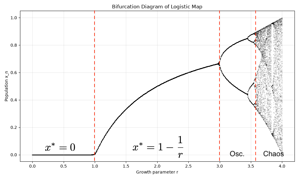
From stability to oscillation

As $r$ increases:

• A stable fixed population becomes unstable.
• The population begins alternating between two values.
• Then four values.
• Then eight.
• Eventually the motion becomes irregular.

This sequence is called period doubling:

$$1 \rightarrow 2 \rightarrow 4 \rightarrow 8 \rightarrow \cdots$$

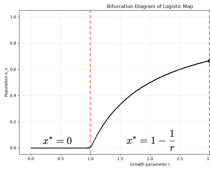
The bifurcation diagram

For each $r$:

1. Choose an initial condition $x_0$.
2. Iterate many times to remove the transient behavior.
3. Plot the next several values of $x_n$.
4. Repeat for many values of $r$.

Deterministic chaos

In the chaotic regime, two nearby initial populations

$$x_0 \qquad\text{and}\qquad x_0+\epsilon$$

can eventually produce very different trajectories.

The system is still completely deterministic.

There is no random number generator.

This is deterministic chaos:

simple equations + sensitivity to initial conditions + long-time unpredictability

Three maps, one idea

Newton-Raphson:

$$z_{n+1} = z_n-\frac{f(z_n)}{f'(z_n)}$$

Which fixed point do we reach?

Mandelbrot:

$$z_{n+1}=z_n^2+c$$

Does the orbit remain bounded?

Logistic:

$$x_{n+1}=rx_n(1-x_n)$$

What long-time behavior emerges?

The computational pattern

For each problem:

1. Choose a map $F$.
2. Choose an initial condition.
3. Iterate: $$x_{n+1}=F(x_n).$$
4. Discard transient behavior when appropriate.
5. Classify or visualize the long-time behavior.
6. Repeat over many initial conditions or parameters.

A few lines of code can reveal structures that are very difficult to anticipate analytically.

Takeaways

• An iterative numerical algorithm can be viewed as a dynamical system.
• Fixed points can be attracting or repelling.
• Nonlinear iteration can generate fractal basin boundaries.
• Changing a parameter can cause bifurcations and qualitative changes in behavior.
• Deterministic systems can exhibit chaos and strong sensitivity to initial conditions.

Simple deterministic rules can generate extraordinarily complex behavior.