by Eugeniy E. Mikhailov and Greg Bentsen
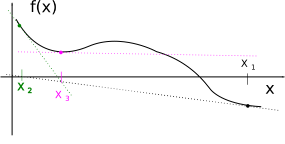
Newton-Raphson and other using estimate of derivative algorithms are usually fast but starting points need to be close enough to the root.
Watch out for
Using root_scalar from scipy.optimize
package
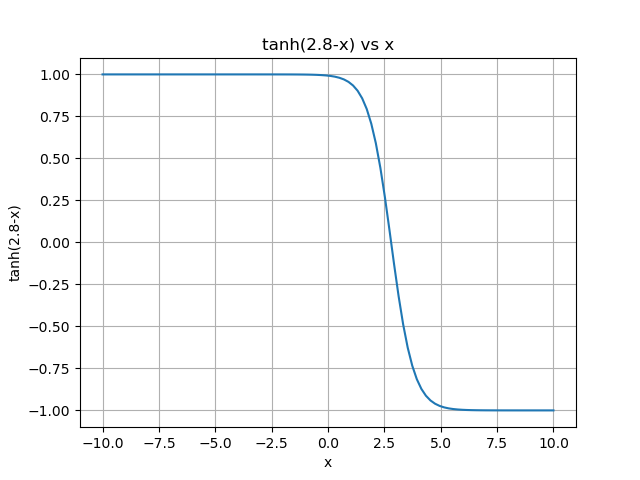
root_scalar(f, args=(), method=None, bracket=None, fprime=None, fprime2=None, x0=None, x1=None, xtol=None, rtol=None, maxiter=None, options=None)See file find_tanh_root.py
import numpy as np
from scipy.optimize import root_scalar
def f(x, *my_arg, **my_kwargs): # note dummy variable needed by root_scalar
return np.tanh(2.8 - x)
In [78]: root_scalar(f, 'newton', x0=2.5)
Out[78]:
converged: True
flag: converged
function_calls: 7
iterations: 3
root: 2.8
method: newton
In [79]: root_scalar(f, 'newton', x0=1)
/usr/lib/python3/dist-packages/scipy/optimize/_root_scalar.py:327:
RuntimeWarning: Derivative was zero.
r, sol = methodc(f, x0, args=args, fprime=fprime, fprime2=None,
Out[79]:
converged: False
flag: convergence error
function_calls: 6
iterations: 3
root: -596803.8420472746
method: newton
In [85]: root_scalar(f, method='bisect', bracket=[1,5])
Out[85]:
converged: True
flag: converged
function_calls: 43
iterations: 41
root: 2.8000000000010914
method: bisect
In [86]: root_scalar(f, method='ridder', bracket=[1,5])
Out[86]:
converged: True
flag: converged
function_calls: 10
iterations: 4
root: 2.8
method: ridderNote that this methods take longer and more function calls. But they always work if bracketed right.
Bracketing algorithm
Non bracketing algorithm
One or more ends of integral have infinity
Solution: do a variable change.
For example
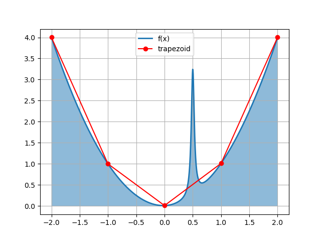
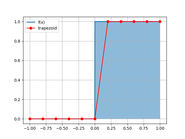
Not enough points
Solution
Simpson and similar methods, which assumes smooth function, will have larger error than seemingly inferior methods
We know that integral exist but numerically it produce infinities, typically because we divide by zero
For example:
We can
skip the small vicinity around singularity
add tiny offset to denominator
The above not always work, since as we will have some problem with the numerical evaluation. For example, Simpson method might not converge.
Alternatively, we can recall that “computer is not substitute for the brain” and do a variable substitution trick
A more useful identity comes from differentiating : Hence, provided ,
Substituting this into the integral,
Applying integration by parts and assuming that on the interval.
see file one_over_sqrt_integral.py where
import numpy as np
import matplotlib.pyplot as plt
from scipy.integrate import quad
from p3_simpson_integration import mysimpson
def u(x):
return x*x
def f_with_E(x, En):
return (En - u(x))
En= 4
f = lambda x: f_with_E(x, En)
sqrtF = lambda x: 1/np.sqrt(f(x))
a= -np.sqrt(En) # technically we need to run root solver
b= np.sqrt(En)
print(f"we expect integral to be pi, i.e. {np.pi}")
resLib = quad(sqrtF, a, b)
print(f"scipy library gives {resLib=}")
Np = 10001
delta=1e-10
resMy = mysimpson(sqrtF, a+delta, b-delta, Np )
print(f"with small limit change Simpson gives {resMy=} for {Np=} and {delta=}")
"""
Now we will do with variable change
note that full integral is 2 * Integral from 0 to b (due to symmetry)
we split this integral 0 to b/2 where there is nothing bad with integrand
"""
int1 = mysimpson(sqrtF, 0, b/2, Np)
# and b/2 to b, where we will do substitution of a variable
def dfdx(f, x, h=1e-6): return (f(x+h) - f(x-h))/(2*h)
def df2dx2(f, x, h=1e-6): return (dfdx(f, x+h, h) - dfdx(f, x-h, h)) /(2*h) # brute force
def g(x):
return np.sqrt(f(x))/ (dfdx(f, x)*dfdx(f, x)) * df2dx2(f, x)
int2 = 2*np.sqrt(f(b))/dfdx(f, b) - 2*np.sqrt(f(b/2))/dfdx(f, b/2) + 2 *mysimpson(g, b/2, b, Np)
resByParts = 2 * (int1 + int2)
print(f"with a variable change trick Simpson gives {resByParts=} for {Np=}")