Logistics and Agenda

• Monday: Monte-Carlo integration
• Tuesday: root finding and integration gotchas
• Friday: mock in-class exam

Midterm 1:

Do it at home part

• Midterm write up and code is due Sunday October 4th 11:59pm
  • there is no late submission option
• You may not use AI to write the report.
  • Report should be done by you and only one per group is needed

In class part

• on Friday October 2nd: mock exam (no grades and you do not even have to do it)
  • check if your computers are battle worthy for off-line use
  • see a typical problem set
• on Monday October 5th, with computers but no AI and no Internet connection
  • we will give you modified assignment which would be similar
  • it will require modification or reuse of prepared code

Toy example - area of the pond

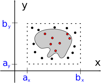
Pond and random hits illustration

$$A_{pond}=\frac{N_{inside}}{N_{total}} A_{box}$$ where $$A_{box} = (b_x-a_x) (b_y-a_y)$$

• Points must be uniformly and randomly distributed across the area.
• The smaller the enclosing box the better it is.

Naive Monte Carlo integration

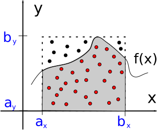
Naive Monte-Carlo setup

$$\int_{a_x}^{b_x} f(x) dx =\frac{N_{inside}}{N_{total}} A_{box}$$ where $$A_{box} = (b_x-a_x) (b_y)$$

• Points must be uniformly and randomly distributed across the area.
• The smaller the enclosing box the better it is. So $max(f(x)) \to b_y$

Monte Carlo integration derived

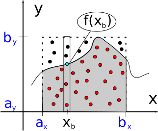
Improved Monte-Carlo setup

Notice that if we choose a small stripe around the bin value $x_b$, then subset of points in that stripe gives an estimate for $f(x_b)$.

Thus why bother spreading points around area?

Let’s chose a uniform random distribution of points ${x_i}$ inside $[a_x, b_x]$

$$\int_{a_x}^{b_x} f(x) dx \approx \frac{b_x - a_x}{N}\sum_{i=1}^N f(x_i)$$

Error estimate for Monte-Carlo method

On the first glance it is horendous method in comaparison even to the box method where $E \sim 1/N$

Monte-Carlo 1D example

import numpy as np
def monte_carlo(func, a, b, N=1_000_000):
    """Monte Carlo Integration"""
    xi = np.random.uniform(a, b, N)
    f_xi = func(xi)
    return np.mean(f_xi) * (b - a)

if __name__ == "__main__":
    import matplotlib.pyplot as plt
    def f(x):
        return x * x
    a = 0
    b = 1
    Np = 100  # hom many points to plot
    N = np.logspace(1, 6, Np, dtype=np.int64)  # used in Monte-Carlo
    integral_for_N = np.zeros(Np)
    for i, n in enumerate(N):
        integral_for_N[i] = monte_carlo(f, a, b, n)

    plt.loglog(N, np.abs(integral_for_N - 1 / 3))
    plt.grid(True)
    plt.xlabel("N")
    plt.ylabel("Deviation from true value")
    plt.savefig("monte_carlo_deviation.png")

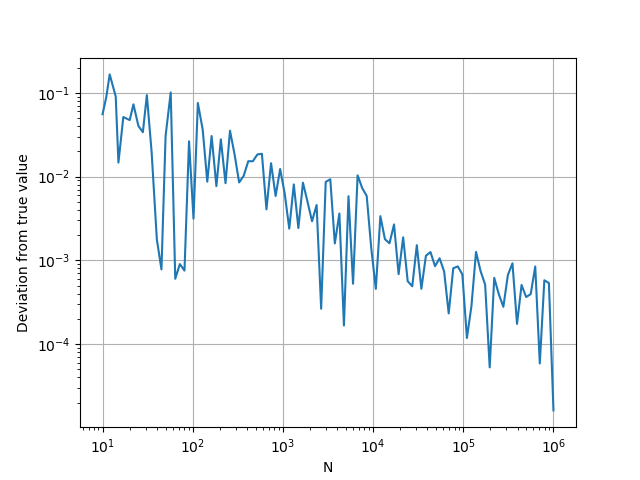
Scaling of Monte-Carlo algorithmic error

Multidimensional integration with interval splitting

$$\int_{a_x}^{b_x} \int_{a_y}^{b_y} f(x,y) ~ dx ~ dy = \int_{a_x}^{b_x} dx \int_{a_y}^{b_y} dy ~ f(x,y)$$

Note that last integral is the function of only $x$

Thus we replaced multidimensional integral as consequent series of single dimension integrals, which we already know how to do.

3D case would look like this

$$\int_{a_x}^{b_x} \int_{a_y}^{b_y} \int_{a_z}^{b_z} f(x,y,z) ~ dx ~ dy ~ dz = \int_{a_x}^{b_x} dx \int_{a_y}^{b_y} dy \int_{a_z}^{b_z} dz ~ f(x,y,z)$$

Multidimensional integration with Monte Carlo

Note that if we would like to split integration region by $N$ points in every of $D$ dimensions, then evaluation time grows $\sim N^D$, which renders Rectangle, Trapezoidal, Simpson, and alike methods useless.

Monte Carlo method is a notable exception, it looks very simple even for multidimensional case and maintains the same $\sim N$ evaluation time.

3D case would look like this

$$\int_{a_x}^{b_x} dx \int_{a_y}^{b_y} dy \int_{a_z}^{b_z} dz ~ f(x,y,z) \approx \frac{ (b_x - a_x) (b_y - a_y) (b_z - a_z) }{N}\sum_{i=1}^N f(x_i, y_i, z_i)$$

A general case

$$\int_{V} dV ~ f(\vec{x}) = \int_{V} dx_1 dx_2 dx_3 ... dx_D ~ f(\vec{x}) \approx \frac{V}{N} \sum_{i=1}^N f(\vec{x}_i)$$

where V is the multidimensional volume , ${\vec{x}_i}$ randomly and uniformly distributed points in the volume V.