Logistics and Agenda

Midterm 1:

Do it at home part

• Midterm write up and code is due Sunday October 4th 11:59pm

• You may use AI freely to write code, debug, and test.

• You are responsible for the code you submit.

• We expect you to understand what the code is doing.

• You may not use AI to write the report.

  • Report should be done by you and only one per group is needed

In class part

• on Monday October 5th, with computers but no AI and no Internet connection
  • we will give you modified assignment which would be similar
  • it will require modification or reuse of prepared code

The Riemann sum

Recall the Riemann integral definition our goal is to find

$$\int_a^b f(x) dx = \lim_{N \to \infty} \sum_{i=1}^{N-1} f(x_i) h$$

where $N$ is the number of points, $h=(b-a)/(N-1)$ is the distance between points.

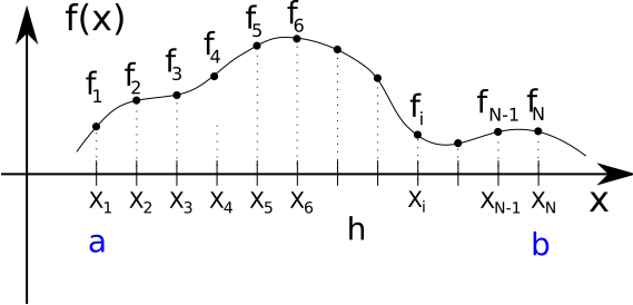
Function under integral

The Rectangle (box) method

Riemann rule is almost direct recipe for the rectangle left end method

$$\int_a^b f(x) dx \approx \sum_{i=1}^{N-1} f(x_i) h$$ where $h=\frac{b-a}{N-1}$ and $x_i=a+(i-1)h$

We just need to remember about round off errors so $h$ should not be too small or equivalently $N$ should not be to big.

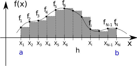
Rectangle left end method

Trapezoidal method

$$\int_a^b f(x) dx \approx h \times (\frac{1}{2} f_1 + f_2 +f_3 + \cdots +f_{N-2} +f_{N-1} + \frac{1}{2} f_{N}) = h \sum_{i=1}^N f(x_i) w_i$$

where $h=\frac{b-a}{N-1}$ and $x_i=a+(i-1)h$

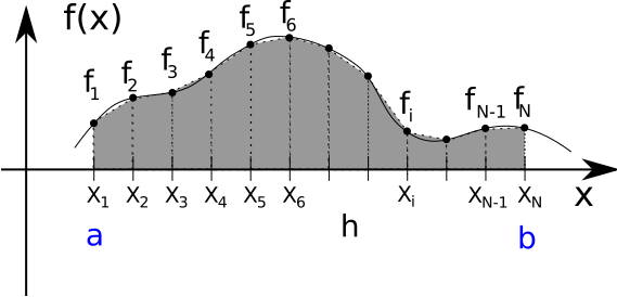
Trapezoid method

Let’s compare implementation of trapezoidal method

# AI generated code

def trapezoidal_ai(func, a, b, Np):
    """
    Numerical integration using the trapezoidal rule.

    Parameters:
    func: function to integrate
    a: lower limit of integration
    b: upper limit of integration
    Np: number of points (intervals = Np - 1)

    Returns:
    Approximation of the integral
    """

# Calculate step size

h = (b - a) / (Np - 1)

# Evaluate function at endpoints

integral = 0.5 * (func(a) + func(b))

# Sum the interior points

for i in range(1, Np - 1):
        x = a + i * h
        integral += func(x)

# Multiply by step size

integral *= h

    return integral

# human generated code

import numpy as np

def trapezoidal_human(func, a, b, Np):
    """Numerical integration using the trapezoidal rule."""
    h = (b - a) / (Np - 1)

    x = np.linspace(a, b, Np)
    y = func(x)
    y[0] = y[0] / 2
    y[-1] = y[-1] / 2

    return np.sum(y) * h

Simpson method: approximation by parabolas.

Main idea take two adjacent points $f_{k-1}$, $f_{k}$, and $f_{k+1}$ and approximate the $f(x)$ by parabola on this $2h$ interval. Then the integral on this interval is approximated as $\frac{h}{3} (f_{k-1} + 4f_{k} + f_{k+1})$

$$\int_a^b f(x) dx \approx h \frac{1}{3}\times ( f_1 + 4 f_2 + 2 f_3 + 4 f_4 + \cdots +2 f_{N-2} +4 f_{N-1} + f_{N}) = h \sum_{i=1}^N f(x_i) w_i$$

where $h=\frac{b-a}{N-1}$ and $x_i=a+(i-1)h$

Note that N must be in special form N=2k+1, i.e. odd.

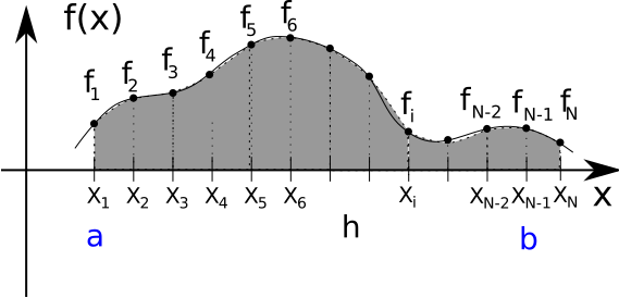
Simpson method

Integration error estimate

Rectangle method $$E={\mathbf{O}}\left( \frac{ (b -a) h}{2} f' \right) = {\mathbf{O}}\left( \frac{ (b -a)^2}{2 N} f' \right)$$

Trapezoidal method $$E={\mathbf{O}}\left( \frac{ (b -a) h^2}{12} f'' \right) = {\mathbf{O}}\left( \frac{ (b -a)^3}{12 N^2} f'' \right)$$

Simpson method $$E={\mathbf{O}}\left( \frac{ (b -a) h^4}{180} f^{(4)} \right) = {\mathbf{O}}\left( \frac{ (b -a)^5}{180 N^4} f^{(4)} \right)$$

Library method for numerical integration

use quad from scipy.integrate module

import scipy.integrate as integrate

def f(x): return x*x
int_estimate, error_estimate = integrate.quad(f, 0, 1)

In [2]: int_estimate
Out[2]: 0.33333333333333337

In [3]: error_estimate
Out[3]: 3.700743415417189e-15