Logistics and Agenda

Homework 3 due Monday Sept 21 at 11:59pm

Agenda

• This week:  Data reduction & fitting, AI tools
• Next week:  Root-finding, numerical integration

Today

• Quiz (10 min)
• Data reduction & fitting basics

AI Tools Installation

We will begin using AI tools this Wednesday

We have set up a local model in the HPC cluster for the class to use.

Please set up the AI tool ASAP. We will expect you to have it set up prior to class on Wednesday.

If you have any trouble please come to our office hours

AI Tools Instructions

Visit this link:

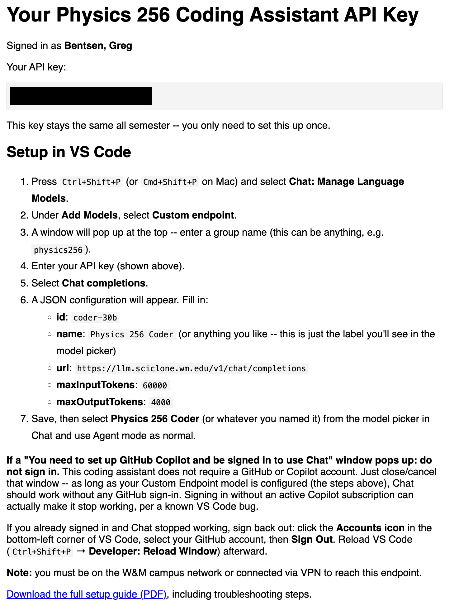
https://hpc.wm.edu/apikey/

Data reduction

• Typical modern experiments generate a huge amount of data.
• There is no way for a human to comprehend all of it.

Data reduction

• Typical modern experiments generate a huge amount of data.
• There is no way for a human to comprehend all of it.

• We need to post-process the data to extract important parameters.
• We might also want to check how our models reflect reality.

Model extraction — fitting

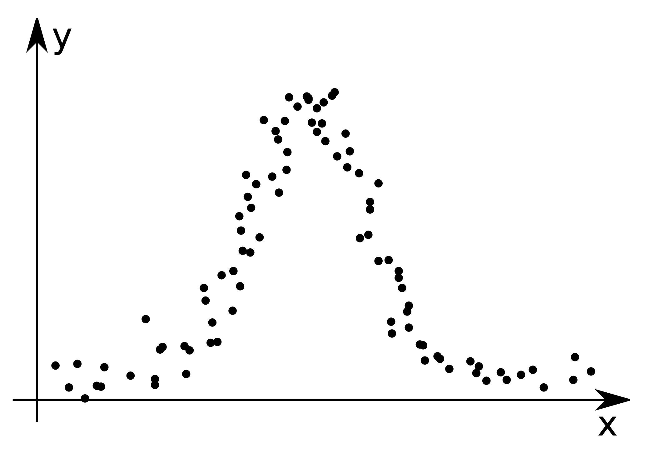
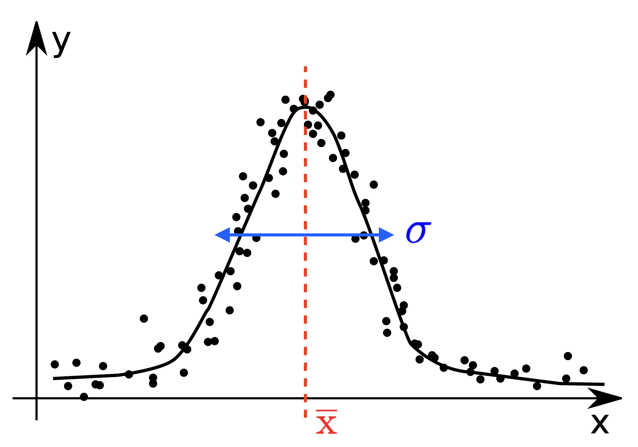
Suppose we measured the dependence of an experimental parameter $y$ on another parameter $x$, yielding a set of $N$ datapoints $\{x_i, y_i\}$.

We have a model $f(x,\vec{p})$ that aims to predict the $y$-values based on the $x$-values, i.e.

$$y_{i,\text{pred}} = f(x_i,\vec{p})$$

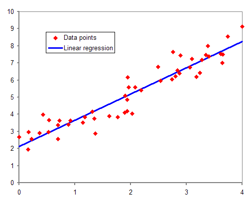
For example, this could be a simple linear model: $f(x, \vec{p}) = m x + b$ with $\vec{p} = (m,b)$.

Source: https://commons.wikimedia.org/w/index.php?curid=3337769

Model extraction — fitting

Suppose we measured the dependence of an experimental parameter $y$ on another parameter $x$, yielding a set of $N$ datapoints $\{x_i, y_i\}$.

We have a model $f(x,\vec{p})$ that aims to predict the $y$-values based on the $x$-values, i.e.

$$y_{i,\text{pred}} = f(x_i,\vec{p})$$

For example, this could be a simple linear model: $f(x, \vec{p}) = m x + b$ with $\vec{p} = (m,b)$.

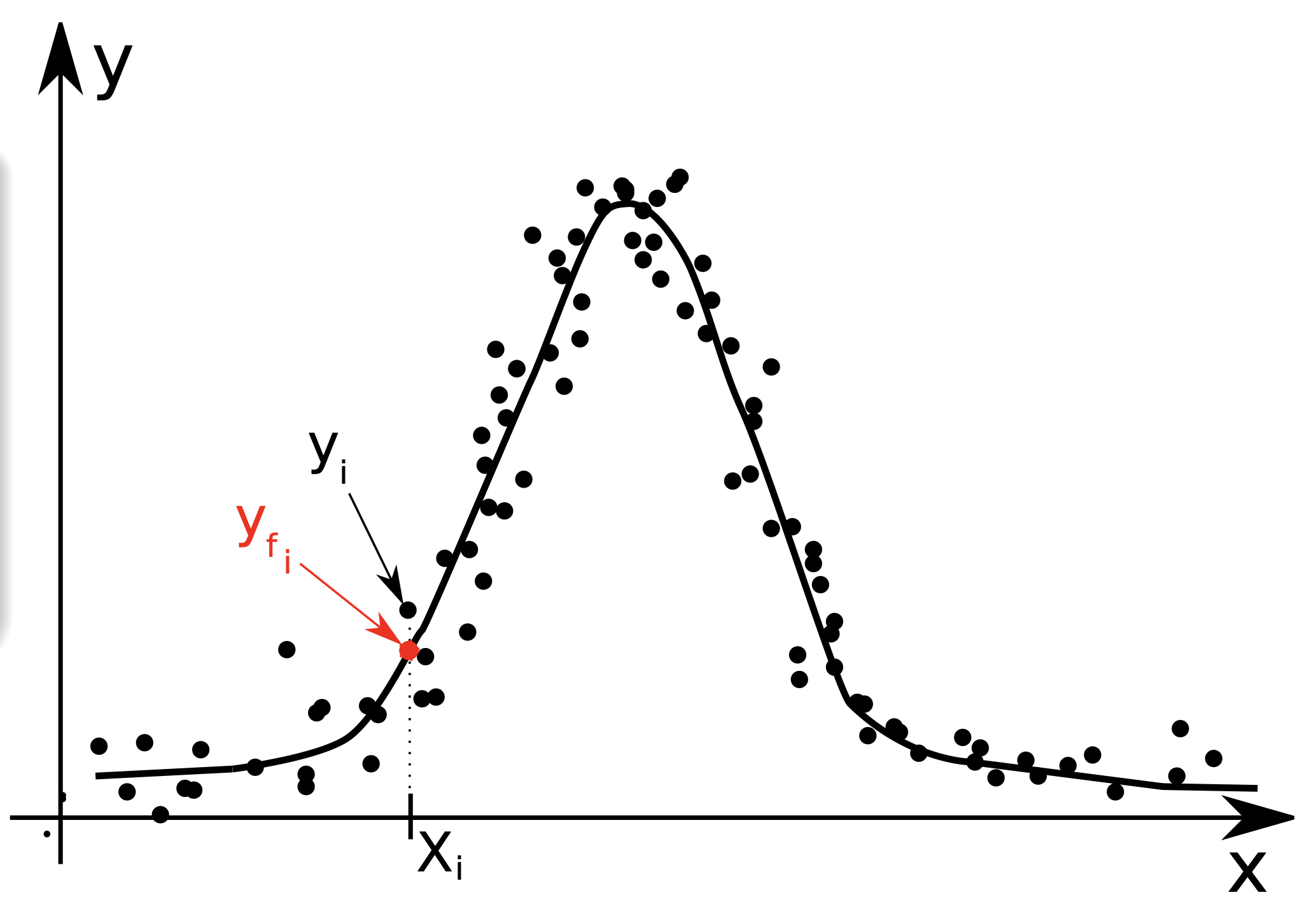
Goal:  We want to extract the unknown model parameters $p_1, p_2, p_3, \ldots = \vec{p}$ (i.e. find the best parameters $\vec{p}$) by fitting the model function $f(x,\vec{p})$ to the data.

• In general $x$ and $y$ could be vectors (multi-dimensional).
• For simplicity, focus on the one-dimensional case.

Goodness of the fit

Define a way to estimate the goodness of fit.

• Use the chi-squared test: $\chi^2 = \sum_i (y_i - y_{i,\text{pred}})^2$.
• Differences $(y_i - y_{i,\text{pred}})$ are called residuals.
• For a given set of data $\{(x_i, y_i )\}$ and model $f(x,\vec{p})$, the goodness of fit parameter $\chi^2$ depends only on the model parameters $\vec{p}$.

Our goal is simple: find the optimal parameters $\vec{p}$ that minimize $\chi^2$ (least-squares fit).

Good fit should have the following properties

• The model $f(x,\vec{p})$ should use the smallest possible set of parameters $\vec{p}$.
  • With enough fitting parameters you can make every residual zero!
  • But this is unphysical: all data has uncertainties and noise in the measurements
• For a good fit, the residuals should be randomly scattered around zero.
  • i.e. There should be no visible trends in residuals versus $x$.
• The standard deviation of the residuals $= \sqrt{\sum_i (y_i - y_{i,\text{pred}})^2 / N}$ should be on the order of the experimental uncertainty $\Delta y$.
  • This condition is often overlooked but you should keep your eyes on it.
  • It can also give you an estimate of the experimental error bars.
• The fit should be robust: new points should not significantly change the fitted parameters.
• Avoid high-order polynomial fits unless there is a strong physical reason.
  • A line is good; a parabola maybe; higher orders only when justified physically.

Practical realization

• Use curve_fit function from the SciPy optimize library.
• Example model: $$f(x,\vec{p}) = \frac{A}{1 + \left(\frac{x - x_0}{\gamma}\right)^2} \quad \quad \quad \quad \vec{p} = (A, x_0, \gamma)$$.

Example code

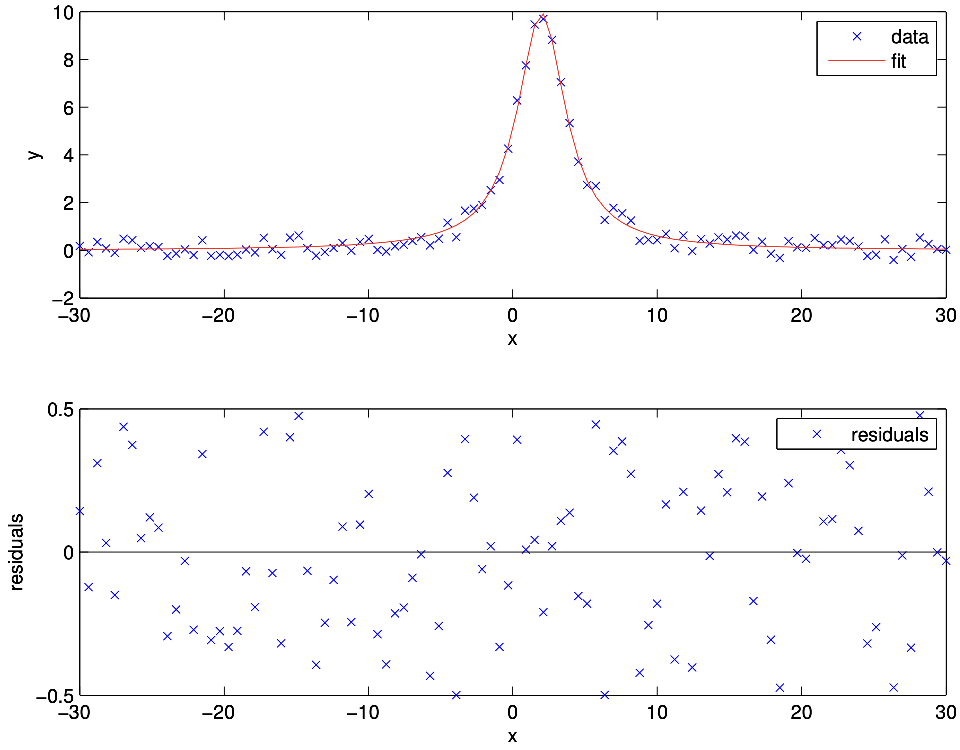
Example fitting code using curve_fit

import numpy as np
import matplotlib.pyplot as plt
from scipy.optimize import curve_fit

# Define Lorentzian function
def lorentzian(x, A, x0, gamma):
    return A / (1 + ((x - x0) / gamma) ** 2)

# Load experimental data
data = np.loadtxt('lorentzian_data.csv', delimiter=',', skiprows=1)
x_data = data[:, 0]
y_data = data[:, 1]

# Initial guess for the parameters [A, x0, gamma]
initial_guess = [10.0, 2.0, 1.0]

# Fit the Lorentzian function to the data
popt, pcov = curve_fit(lorentzian, x_data, y_data, p0=initial_guess)

# Extract fitted parameters
A_fit, x0_fit, gamma_fit = popt

# Plot the resulting fit
x_fit = np.linspace(-30, 30, 1000)
y_fit = lorentzian(x_fit, A_fit, x0_fit, gamma_fit)

plt.figure(figsize=(10, 6))
plt.scatter(x_data, y_data, label='Data', alpha=0.7)
plt.plot(x_fit, y_fit, 'r-', linewidth=2, label='Fit')
plt.savefig('lorentz_fit.png')
plt.show()

Fitted parameters and uncertainty

We obtain two return values from curve_fit:

• popt = the optimal parameter values $\vec{p} = (p_1, p_2, p_3, \ldots)$
• pcov = the covariance matrix for the parameters

The diagonal elements of pcov give you the variances $\text{Var}(p_i)$ of the parameters $p_i$.

To find the uncertainty, just take the square root: $\Delta p_i = \sqrt{\text{Var}(p_i)}$

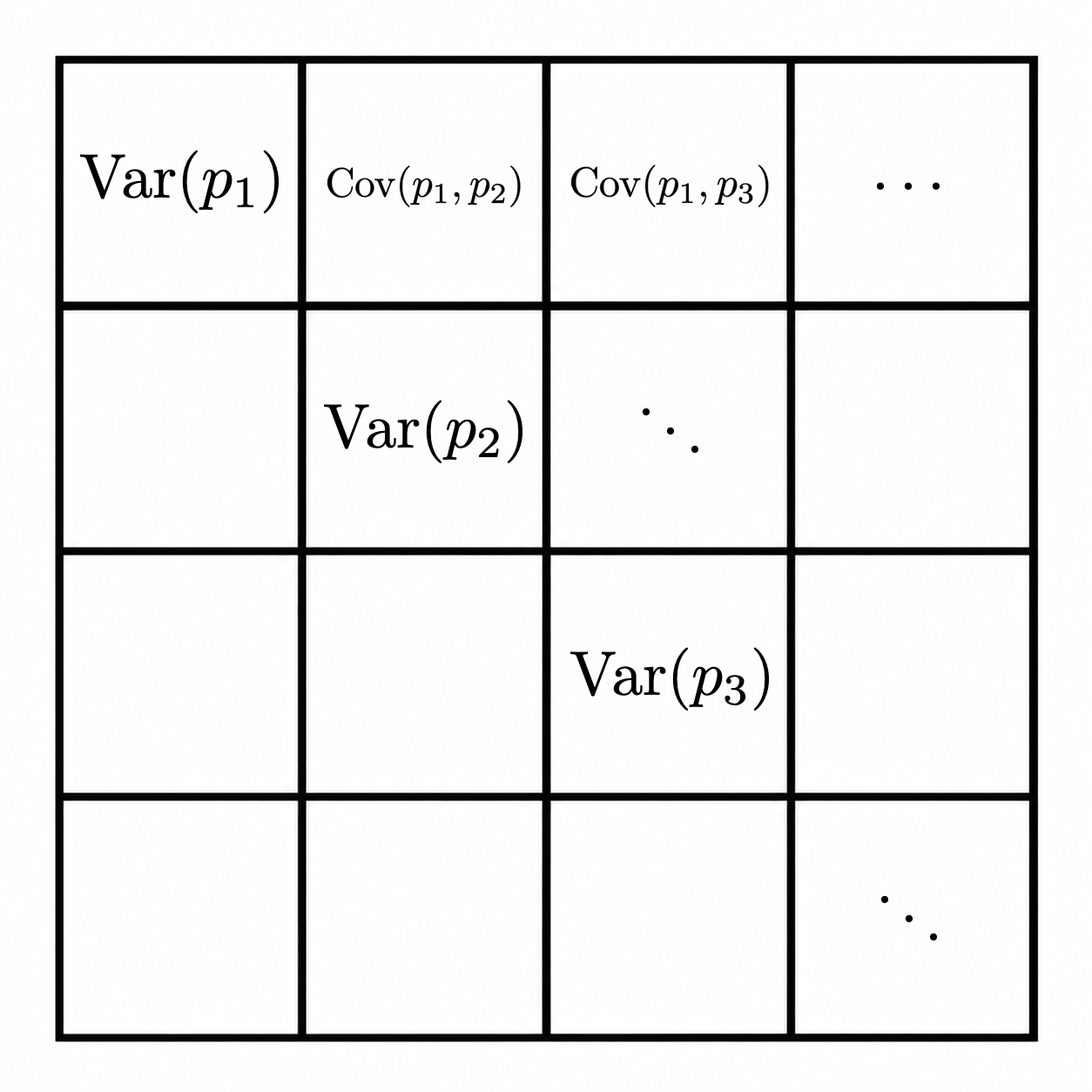
Covariance matrix pcov

See https://en.wikipedia.org/wiki/Covariance_matrix for more information