Functions and scripts
Boolean algebra, conditional statements, loops.
by Eugeniy E.
Mikhailov and Greg
Bentsen
Loops examples
Scripts and functions
Scripts
Script is the sequence of the Python expressions written in the file.
So far we typed them directly to the python prompt.
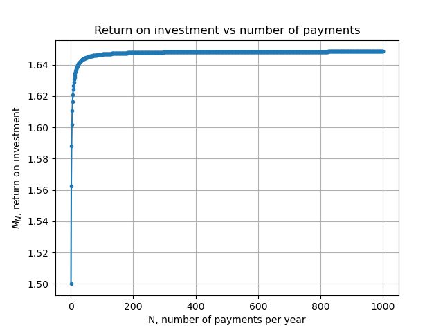
import numpy as np
Nmax = 1000
M = np.zeros(Nmax)  # we need to preallocate space
x=0.5
allN = range(1, Nmax+1)
for N in allN:
    M[N-1] = np.pow(1+x/N, N)  # position in array starts from 0!

import matplotlib.pyplot as plt
plt.plot(allN, M, '.-')
plt.grid(True)
plt.xlabel("N, number of payments per year")
plt.ylabel("$M_N$, return on investment")  # Note it understands LaTeX!
plt.title("Return on investment vs number of payments")
plt.savefig("return_on_investment.png")
Let’s save it to the file plot_return_on_investment.py.
Now we can edit the file and assign any x and
Nmax.
To execute the script directly in the shell
> python plot_return_on_investment.py
There is no visible output, but the figure regenerated.
Alternatively, we can run our script within ipython
itself!
In [1]: %run plot_return_on_investment.py
will not work in python
Now we are free to massage our script to satisfy our needs.
Scripts variable space
Unlike functions scripts modify Workspace
variables
import numpy as np
Nmax = 1000
M = np.zeros(Nmax)  # we need to preallocate space
x=0.5
allN = range(1, Nmax+1)
for N in allN:
    M[N-1] = np.pow(1+x/N, N)  # position in array starts from 0!

import matplotlib.pyplot as plt
plt.plot(allN, M, '.-')
plt.grid(True)
plt.xlabel("N, number of payments per year")
plt.ylabel("$M_N$, return on investment")  # Note it understands LaTeX!
plt.title("Return on investment vs number of payments")
plt.savefig("return_on_investment.png")
In [1]: Nmax=22
In [2]: %run plot_return_on_investment.py
In [3]: Nmax
Out[3]: 1000
See that Nmax value is changed
Think about the script as it is a keyboard macro. Calling a script is
equivalent to typing the scripts statements from the keyboard.
Functions
Python functions
Used for separation of a meaningful chunk of code
def function_name(arg1, arg2, arg3, ..., argN, karg1=val1, karg2=val2, ..., kargN=valN)
    """Optional but super handy doc string"""
    # body of the function
    # notice the indentation!
    .
    .
    return (ret1, ret2, ret3, ... , retN)
- All
args, kargs, and rets are
optional and defined as needed.
- There is also a way to make a function with arbitrary number of
options or arguments
- but this is advance topic
- if you wonder about example,
print function is a good
example
- Function can be typed at the python prompt directly
- Or collections of functions could be saved in file or files
- in this case we call such collections modules, packages, or
libraries
Example of a function definition
In [5]: def minmax(n1, n2=0):
   ...:     """Take two numbers and return them in ascending order.
   ...:        The second argument is optional, if not provided 0 will be used.
   ...:     """
   ...:     if n1 < n2:
   ...:         return (n1, n2)  # this is actually one value, i.e. *tuple* of 2 numbers
   ...:     else:
   ...:         return (n2, n1)
   ...:     # note that python will never reach this point
   ...:

In [6]: minmax(23)
Out[6]: (0, 23)

In [7]: minmax(4, -2)
Out[7]: (-2, 4)

In [8]: minmax(1, 5)
Out[8]: (1, 5)
We can also ask documentation about our function
In [15]: minmax?
Signature: minmax(n1, n2=0)
Docstring:
Take two numbers and return them in ascending order.
The second argument is optional, if not provided 0 will be used.
File:      ~/jobs/wm/2026.fall_practical_computing_for_scientists_256/lecture03/plots_python/<ipython-input-14-a8b09f68fc26>
Type:      function
Local space of variables in functions
Unlike scripts, functions leave Workspace intact.
There are exceptions, in particular in numpy
world!
# Recall that Signature: minmax(n1, n2=0)
>>> n2=33
>>> n1=10
>>> mininmax(10)
What we will get back?
Reusing variables which exist in workspace considered bad idea
In [6]: def f(x):
   ...:     print(n)  # notice that we did not provide n as an argument
   ...:     return x
In [7]: f(3)
---------------------------------------------------------------------------
NameError                                 Traceback (most recent call last)
Cell In[7], line 1
----> 1 f(3)

Cell In[6], line 2, in f(x)
      1 def f(x):
----> 2     print(n)
      3     return x

NameError: name 'n' is not defined
In [8]: n=111

In [9]: f(3)
111
Out[9]: 3
In big projects this “feature” is very prone to run out of control!
Recursion: function calls itself
Canonical example: factorial
We can rewrite it as
Notice that
In [10]: def fact(n):
    ...:     if n <= 1:
    ...:         return 1
    ...:     return n * fact(n-1)
    ...:

In [11]: fact(3)
Out[11]: 6

In [12]: fact(5)
Out[12]: 120
While certain code will look more elegant with recursion, there is a
hard limit for number of the recursive
calls.
Also generally such code is slower than if you can implement it with
loops.
Example: calculating
via Taylor expansion
You might ask how computer calculates
?
One way is to do it by approximating value of
via Taylor expansion
import math
import numpy as np

def mysin(x, N=10):
    s=0
    for n in range(0,N+1):
        s = s + np.pow(-1.0, n) * np.pow(x, 2*n+1) / math.factorial( 2*n +1)
        # we could have use our own factorial implementation as well
        # notice that direct use of factorial is *bad* idea
        # since as n grows, it has to recaluclate same things (n-1)! again and again
        # it would be better to rethink it
        # There is incoming problem for large n! factorial overflow the float representation
    return s
>>> mysin(math.pi)
np.float64(1.0348185903053497e-11)

>>> mysin(math.pi, N=50)
np.float64(3.3280566969799443e-16)

>>> mysin(math.pi/2)
np.float64(1.0000000000000002)

>>> mysin(math.pi/2, N=50)
np.float64(1.0000000000000002)
Spoiler, this is not how trig functions are calculated for arbitrary
.
Usually, via trig identities
brought to the smallest usable value and then it is calculated. Recall
that expansion requires the least members of the sum the close
to 0 (since our equation was expansion of
around 0.
Comparing our mysin implementation to the
numpy.sin one
import numpy as np
import matplotlib.pyplot as plt

x = np.linspace(0, 2*np.pi, 100)  # we create 100 equidistant points
y_numpy_sin = np.sin(x)  # calculate sin for all points of array in  one go

# unfortunately mysin cannot work with array so we have to loop over x values
y_mysin = x*0  # preallocating array
for idx, xp in enumerate(x):
    y_mysin[idx] = mysin(xp)

plt.figure(1)
plt.clf()
plt.plot(x, y_numpy_sin, label='numpy sin')
plt.plot(x, y_mysin, label='my sin')
plt.legend()
plt.grid(True)
plt.xlabel("Angle (rad)")
plt.ylabel("$\sin$ value")
plt.title("Comparison of numpy and our own $\sin$ calculations")

plt.figure(2)
plt.clf()
plt.plot(x, y_numpy_sin-y_mysin, label='difference')
plt.grid(True)
plt.legend()
plt.xlabel("Angle (rad)")
plt.ylabel("np.sin(x) - mysin(x)")
plt.title("Comparison of numpy and our own $\sin$ calculations")
Now we know enough of python to be dangerous do useful
work
By now we completed equivalent of CSCI 141 class :) The rest is
mastering what we know.
What did we skip? Quite a
lot.
The major omitted pieces
We will talk about them as needed or avoid them completely. After all
numerical computations usually do not require fancy things.
The sliver of python iceberg can be seen in python tutorial.