Creating Graphs in MATLAB

You first have to get your data into MATLAB. You can do this in one of two ways: 1) Input the data manually. or 2) Import data from a file.

To input data manually, choose File > New > Variable. Give this new variable a name. It will appear in your workspace. You can double-click on this variable to open up an Array Editor, which is reminiscent of Microsoft Excel. Input your data in columns.

To import data from a file choose File > Import Data.... This brings up the Import Wizard:

1. Find file in "Current Directory" window. Use "up-folder" button to find other folders on the computer. Select the correct folder and the correct file.

2. Right click and select "Import Data..."

3. Change "Number of text header lines:" (top right of window) to 7 (or to the number of lines in the header of the current file).

4. Click "Next."

5. Right-click "data" and select "Rename Variable" (choose unique_name for data set).

6. Click "Finish."

7. Click "Command Window" to get cursor for typing.

8. Type "x_unique_name = unique_name(1:2500,1);" to set the data in the x-axis as a variable (column 1 of the unique_name data set).

9. Type "y_unique_name = unique_name(1:2500,2);" to set the data in the y-axis as a variable (column 2 of the unique_name data set).

The unique name is whatever the user specifies; a common way to name is to set the data as the file number.

MATLAB deals with matrices. Let's say you have your data in the columns of a 22x2 matrix that you've loaded into your workspace. you can get the vectors of data points that you want to plot like this:

firstset = data(1:22,1);

secondset = data(1:22,2);

Note the syntax: matrixname(beginRow# : endRow# , column#).

Use the semi-colon to suppress output. You will see these new variables in your Workspace Window .

If you want to make a plot of the data with x=first set, y=second set, do this:

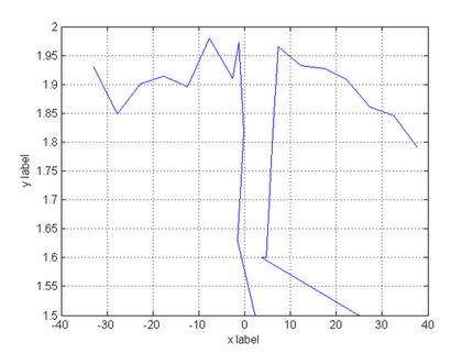
p1 = plot(firstset, secondset);xlabel('x label');ylabel('y label');grid on

A figure will pop up. other options are to use scatter instead of plot

With the figure open, you can select the Property Editor from the View menu and change the tick marks, title, legend, etc.

Notice that the default y-range isn't really nice. We can change this with the following command:

ylim([1,2])

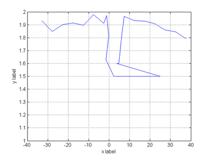
Let's say that we want to change our x-grid to something finer. The following command places ticks from x=-40 to x=+40 at intervals of 5. The command gca returns the current options for the axes. XTick sets new values for that specific property.

set(gca,'XTick',-40:5:40)

You can also perform some Basic Fitting from the Tools menu. This is one of the more straight-forward MATLAB tools. Simply select the type of fit that you want and whether you want to display the equation on the figure.

If the fitting function you need is not available in the Basic Fitting menu, or you need to fit only a part of the data set, the procedure is different:

To plot the data:

1. Click "Start" at the bottom left corner of Matlab window, and highlight "Toolboxes" and then "Curve Fitting."

2. Click on "Curve Fitting Tool" (a new window will open).

3. Click "Data" and select "x_unique_name" for the X Data and "y_unique_name" for the Y Data.

4. Click "Create Data Set" (a plot should appear in the Curve Fitting Tool window).

5. Click "Close."

To select a part of the data set you need to create exclusion rules:

1. Click "Exclude..." in the Curve Fitting Tool window.

2. Type in the "Exclusion Rule Name" box to give the exclusion rule a name.

3. Click the drop down menu beside "Select Data Set" to choose the data set.

4. Click "Exclude Graphically" (a new window will open).

5. To select points, the cursor draws boxes (cannot click a single point). Depending on the size of the range you want to fit, it may be easier to first click "Exclude All" and use the right mouse button to include the range of data that is to be fitted. The zoom-in tool will be necessary to include all the points. Click once to select the zoom, and the second time to de-select the zoom. When finished, click "Close."

6. Click "Create Exclusion Rule" in the "Exclude" window (should appear in the smaller right hand "Existing Exclusion Rules:" window in the "Exclude" window).

7. Click "Close."

What to do if the function you need is not in the list of standard Matlab functions? One solution is to use a Custom Equation. Just note that in this case you will need to adjust initial values for fitting parameters under “Fit Option” button to be fairly close to the correct ones. If initial values are too far, the fit may not converge properly. And Matlab is not good in guessing the initial parameters! Also we found that Levenberg-Marquadt Algorithm provides the best fitting results.

However, if custom equations do not converge properly, you may get creative with the existing standard fitting functions. For example, that is how we ``added’’ an offset to a standard Gaussian fitting function.

1. Click "Fitting..." in "Curve Fitting Tool" window.

2. Click "New Fit."

3. Click the drop down menu beside "Data Set" to choose the proper data set.

4. Click the drop down menu beside "Exclusion Rule" to choose the exclusion rule.

5. Click the drop down menu beside "Type of Fit" to choose Gaussian.

6. Click on the second Gaussian choice, "a1*exp(-((x-b1)/c1)^2) + a2*exp(-((x-b2)/c2)^2."

7. Click "Fit Options..."

8. Change c2 "StartPoint" from the initial value to 1e10.

9. Click "Close."

10. Click "Apply" (Fit should have offset and mimick the curve that was chosen with the exclusion rule).

11. Repeat with as many exclusion rules that are available for a given plot, clicking "New Fit" each repetition.