---
author:
- "by [Eugeniy E. Mikhailov](http://physics.wm.edu/~evmik/) and [Greg
Bentsen](https://physics.wm.edu/~gbentsen/)"
title: Data reduction & fitting
---
## Logistics and Agenda
Homework 3 due Monday Sept 21 at 11:59pm
\
Agenda
- This week: Data reduction & fitting, AI tools
- Next week: Root-finding, numerical integration
\
Today
- Quiz (10 min)
- Data reduction & fitting basics
## AI Tools Installation
We will begin using AI tools **this Wednesday**
We have set up a local model in the HPC cluster for the class to use.
**Please set up the AI tool ASAP. We will expect you to have it set up
prior to class on Wednesday.**
If you have any trouble please **come to our office hours**
## AI Tools Instructions
Visit this link:
::: {style="text-align: center;"}
{width="50%"}
:::
# Data Reduction & Fitting
## Data reduction
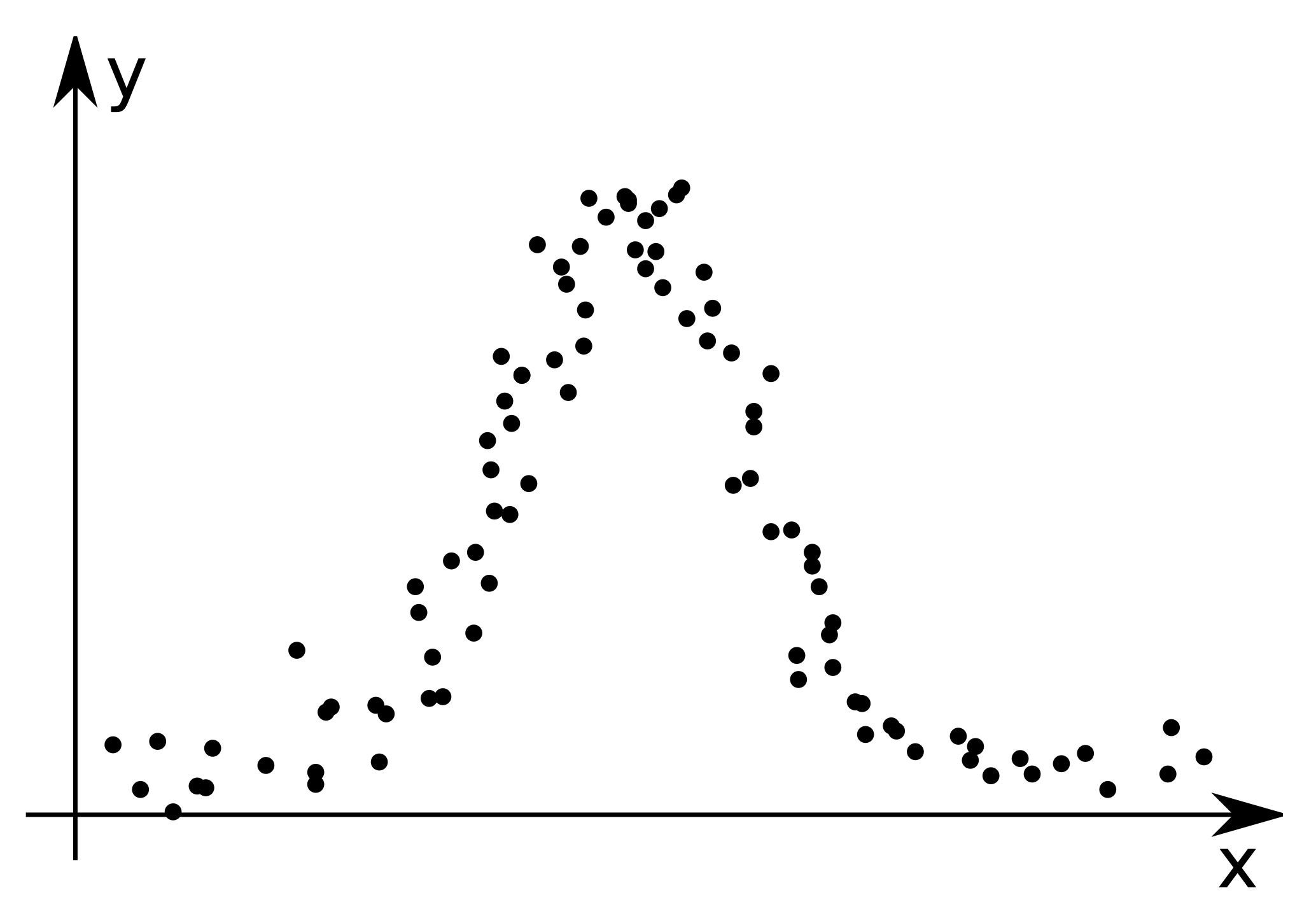
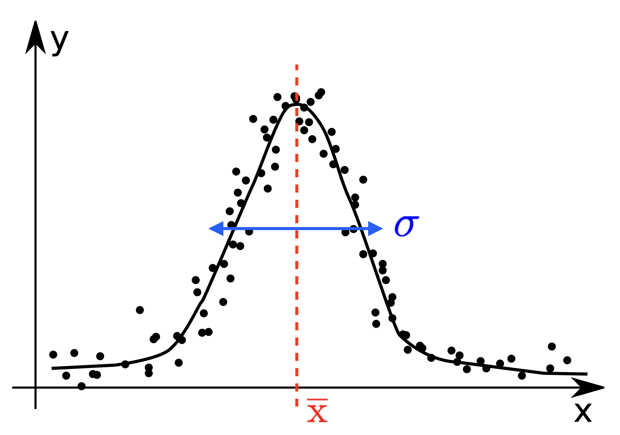
- Typical modern experiments generate a huge amount of data.
- There is no way for a human to comprehend all of it.
::: {style="text-align: center;"}
{width="50%"}
:::
## Data reduction
- Typical modern experiments generate a huge amount of data.
- There is no way for a human to comprehend all of it.
::: {style="text-align: center;"}
{width="50%"}
:::
- We need to post-process the data to extract [important
parameters]{style="color: red;"}.
- We might also want to check how our models reflect reality.
## Model extraction --- fitting
Suppose we measured the dependence of an experimental parameter $y$ on
another parameter $x$, yielding a set of $N$ datapoints $\{x_i, y_i\}$.
We have a **model** $f(x,\vec{p})$ that aims to predict the $y$-values
based on the $x$-values, i.e.
$$y_{i,\text{pred}} = f(x_i,\vec{p})$$
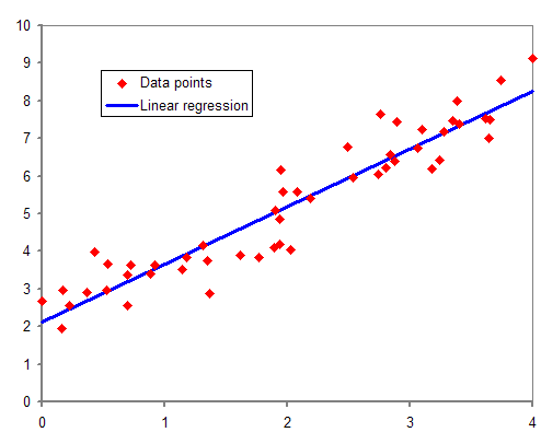
For example, this could be a simple linear model:
$f(x, \vec{p}) = m x + b$ with $\vec{p} = (m,b)$.
::: {style="text-align: center;"}
{width="40%"}
:::
## Model extraction --- fitting
Suppose we measured the dependence of an experimental parameter $y$ on
another parameter $x$, yielding a set of $N$ datapoints $\{x_i, y_i\}$.
We have a **model** $f(x,\vec{p})$ that aims to predict the $y$-values
based on the $x$-values, i.e.
$$y_{i,\text{pred}} = f(x_i,\vec{p})$$
For example, this could be a simple linear model:
$f(x, \vec{p}) = m x + b$ with $\vec{p} = (m,b)$.
\
**Goal:** We want to extract the unknown model parameters
$p_1, p_2, p_3, \ldots = \vec{p}$ (i.e. find the best parameters
$\vec{p}$) by fitting the model function $f(x,\vec{p})$ to the data.
- In general $x$ and $y$ could be vectors (multi-dimensional).
- For simplicity, focus on the one-dimensional case.
## Goodness of the fit
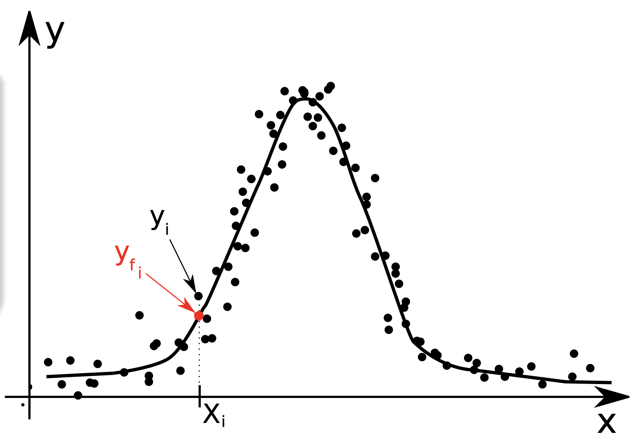
Define a way to estimate the goodness of fit.
- Use the chi-squared test:
$\chi^2 = \sum_i (y_i - y_{i,\text{pred}})^2$.
- Differences $(y_i - y_{i,\text{pred}})$ are called
[residuals]{style="color: red;"}.
- For a given set of data $\{(x_i, y_i )\}$ and model $f(x,\vec{p})$,
the goodness of fit parameter $\chi^2$ depends only on the model
parameters $\vec{p}$.
Our goal is simple: find the optimal parameters $\vec{p}$ that minimize
$\chi^2$ **(least-squares fit)**.
::: {style="text-align: center;"}
{width="50%"}
:::
## Good fit should have the following properties
- The model $f(x,\vec{p})$ should use the smallest possible set of
parameters $\vec{p}$.
- With enough fitting parameters you can make every residual zero!
- But this is unphysical: all data has uncertainties and noise in
the measurements
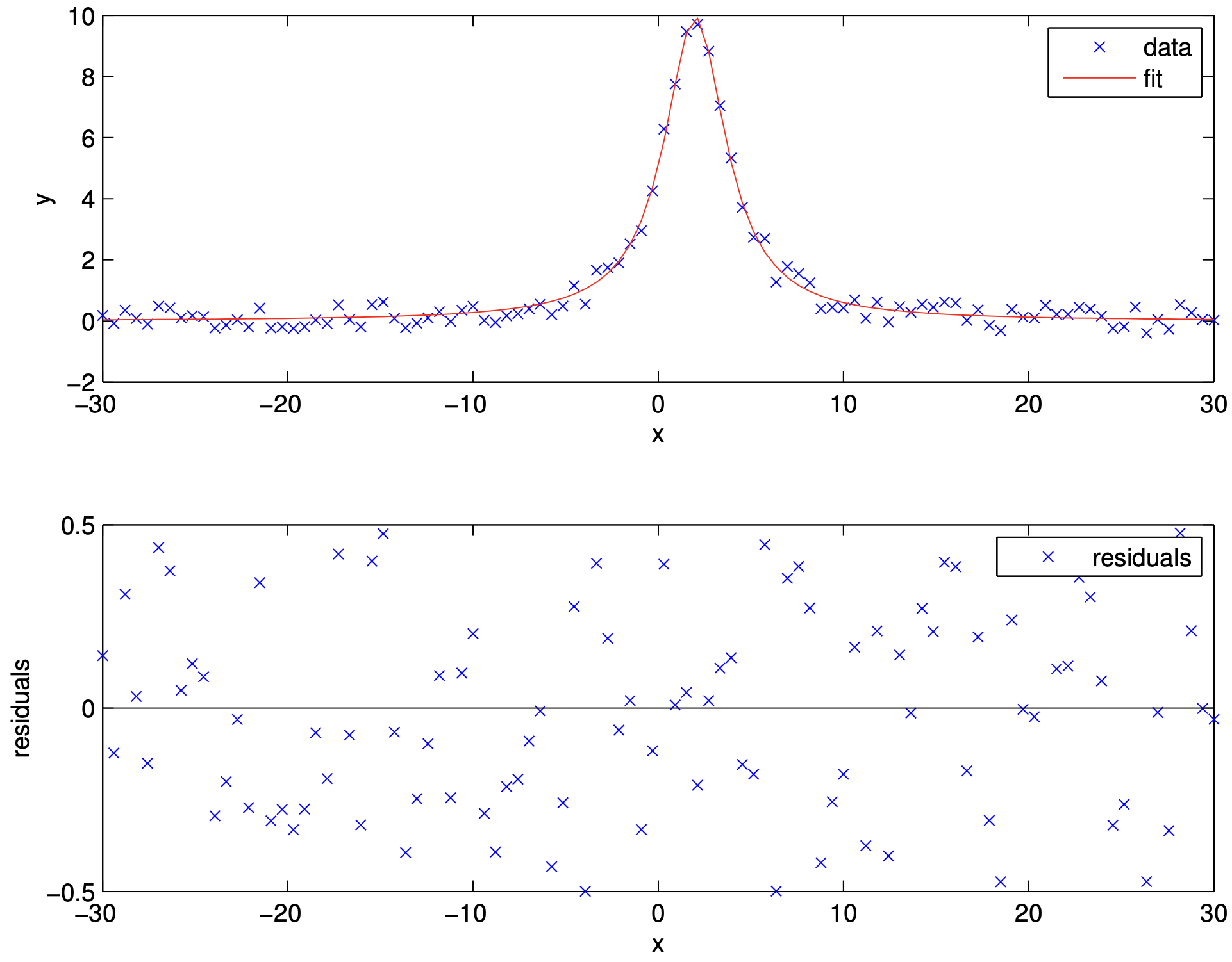
- For a good fit, the residuals should be randomly scattered around
zero.
- i.e. There should be no visible trends in residuals versus $x$.
- The standard deviation of the residuals
$= \sqrt{\sum_i (y_i - y_{i,\text{pred}})^2 / N}$ should be on the
order of the experimental uncertainty $\Delta y$.
- This condition is often overlooked but you should keep your eyes
on it.
- It can also give you an estimate of the experimental error bars.
- The fit should be robust: new points should not significantly change
the fitted parameters.
- Avoid high-order polynomial fits unless there is a strong physical
reason.
- A line is good; a parabola maybe; higher orders only when
justified physically.
## Practical realization
- Use `curve_fit` function from the SciPy `optimize` library.
- Example model:
$$f(x,\vec{p}) = \frac{A}{1 + \left(\frac{x - x_0}{\gamma}\right)^2} \quad \quad \quad \quad \vec{p} = (A, x_0, \gamma)$$.
::: {style="text-align: center;"}
{width="50%"}
:::
## Example code
Example fitting code using `curve_fit`
``` {.python .numberLines}
import numpy as np
import matplotlib.pyplot as plt
from scipy.optimize import curve_fit
# Define Lorentzian function
def lorentzian(x, A, x0, gamma):
return A / (1 + ((x - x0) / gamma) ** 2)
# Load experimental data
data = np.loadtxt('lorentzian_data.csv', delimiter=',', skiprows=1)
x_data = data[:, 0]
y_data = data[:, 1]
# Initial guess for the parameters [A, x0, gamma]
initial_guess = [10.0, 2.0, 1.0]
# Fit the Lorentzian function to the data
popt, pcov = curve_fit(lorentzian, x_data, y_data, p0=initial_guess)
# Extract fitted parameters
A_fit, x0_fit, gamma_fit = popt
# Plot the resulting fit
x_fit = np.linspace(-30, 30, 1000)
y_fit = lorentzian(x_fit, A_fit, x0_fit, gamma_fit)
plt.figure(figsize=(10, 6))
plt.scatter(x_data, y_data, label='Data', alpha=0.7)
plt.plot(x_fit, y_fit, 'r-', linewidth=2, label='Fit')
plt.savefig('lorentz_fit.png')
plt.show()
```
## Fitted parameters and uncertainty
We obtain two return values from `curve_fit`:
- `popt` = the optimal parameter values
$\vec{p} = (p_1, p_2, p_3, \ldots)$
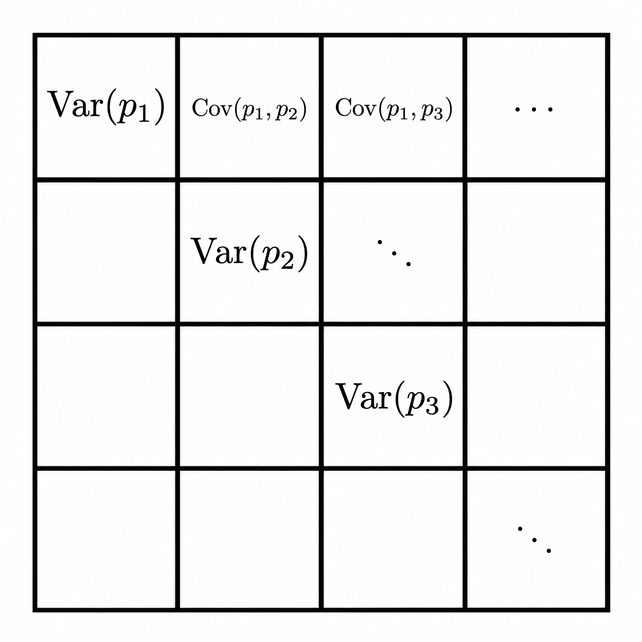
- `pcov` = the covariance matrix for the parameters
\
The diagonal elements of `pcov` give you the variances $\text{Var}(p_i)$
of the parameters $p_i$.
To find the uncertainty, just take the square root:
$\Delta p_i = \sqrt{\text{Var}(p_i)}$
::: {style="text-align: center;"}
{width="25%"}
:::
See for more
information